Reading “Attention Is All You Need”: The Original Transformer Paper

In 2017, Vaswani and seven co-authors, most of them then at Google Brain or Google Research, published Attention Is All You Need and introduced the Transformer. The paper is about machine translation, and its model is an encoder–decoder; most of today’s large language models keep only the decoder half. That context makes the paper easier to read. The authors were asking whether a translation model could do without recurrence and convolution altogether, not how to build a chat model.

What follows goes through the paper in its own order. Section, table and equation numbers refer to arXiv version 7. Worked numerical examples of attention itself are in Attention Mechanism; modern components such as RMSNorm, RoPE, GQA and SwiGLU are covered in Transformers: Original Architecture and Modern Blocks and are not repeated here.

The 2017 Problem: Recurrence Makes Training Wait

Section 1 starts from the state of the art at the time: recurrent networks such as LSTMs and GRUs led in language modelling and machine translation. A recurrent model computes along the sequence one position at a time, producing hidden state $h_t$ from $h_{t-1}$ and the input at position $t$. The authors point out that this inherently sequential computation rules out parallelism within a training example. The problem grows with sequence length, because memory also limits how many examples fit in a batch. Factorization tricks and conditional computation had improved efficiency, but the fundamental constraint of sequential computation remained.

Attention was already a standard part of translation models. It relates two positions directly regardless of their distance, yet it was almost always used together with a recurrent network. The paper proposes removing recurrence entirely and relying on attention alone to draw global dependencies between input and output.

Section 2 sets the Transformer beside another line of work that also reduced sequential computation. The Extended Neural GPU, ByteNet and ConvS2S use convolutions to compute hidden representations for all positions in parallel. In those models, however, the number of operations needed to relate signals from two arbitrary positions grows with their distance, linearly for ConvS2S and logarithmically for ByteNet, which makes distant dependencies harder to learn. The Transformer reduces this to a constant number of operations. The authors name the cost as well: averaging attention-weighted positions reduces the effective resolution, which is what multi-head attention is meant to counteract.

So the paper is after two things at once: how much of training can run in parallel, and how long a path a signal must travel between two distant positions. Table 1 in Section 4 puts both into complexity terms.

The Architecture as the Paper Defines It

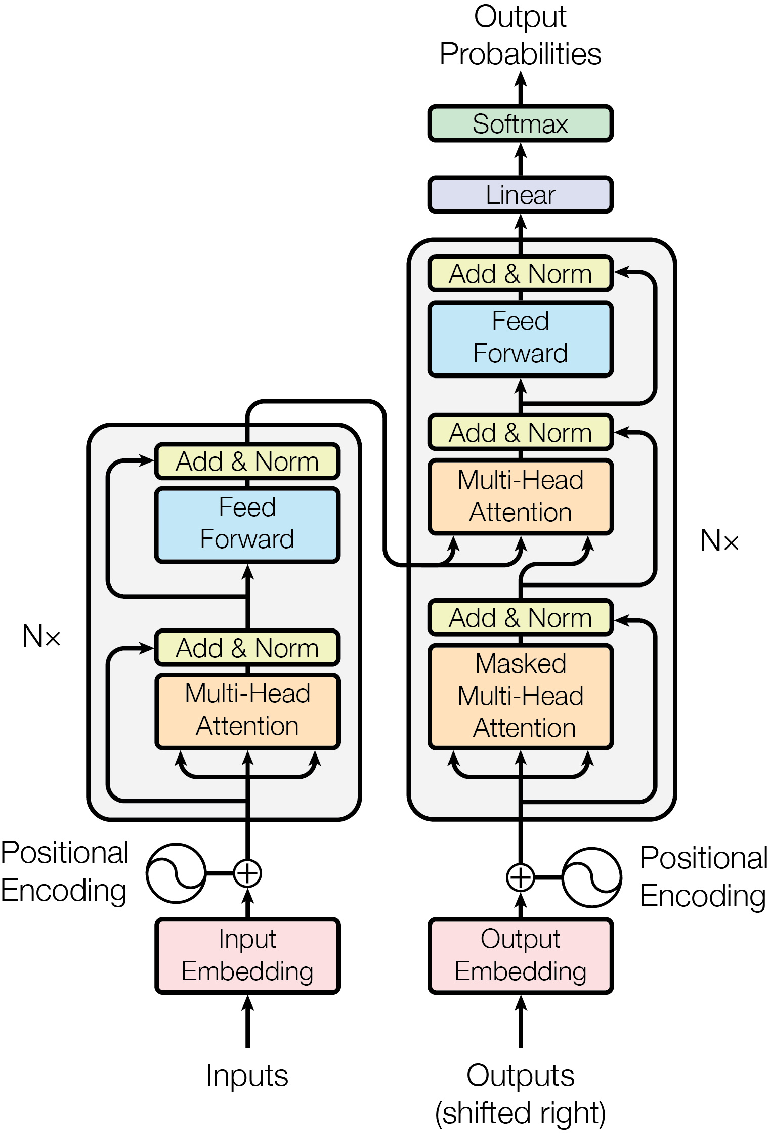
Section 3 keeps the general framework of sequence transduction models. The encoder maps an input sequence of symbols $(x_1,\dots,x_n)$ to continuous representations $\mathbf z=(z_1,\dots,z_n)$. Given $\mathbf z$, the decoder generates an output sequence $(y_1,\dots,y_m)$ one symbol at a time. Each step is autoregressive: the symbols generated so far are fed back as additional input for the next one.

Open full-size image

The encoder is on the left and the decoder on the right; the N× beside each stack means the same layer is repeated $N=6$ times. The arrows that bypass each sublayer are residual connections, and “Add & Norm” means add first, then apply layer normalization. Of the three inputs to the decoder’s middle attention sublayer, two come from the encoder output and one from the decoder itself.

Vaswani et al., Attention Is All You Need (2017), Figure 1. © Google. · Figure reuse permission

Section 3.1 describes the two stacks. The encoder has $N=6$ identical layers, each with two sublayers: multi-head self-attention and a position-wise fully connected feed-forward network. The decoder also has $N=6$ layers and adds a third sublayer, which performs multi-head attention over the output of the encoder stack.

Each sublayer is wrapped in a residual connection followed by layer normalization, so the output of a sublayer is

$$\operatorname{LayerNorm}\big(x+\operatorname{Sublayer}(x)\big).$$

Normalization comes after the residual addition, an ordering later called Post-Norm. To make the residual additions possible, every sublayer and both embedding layers produce outputs of dimension $d_{\text{model}}=512$.

The decoder’s self-attention is masked so that a position cannot attend to later positions. Together with output embeddings shifted right by one position, this ensures that the prediction for position $i$ depends only on known outputs at positions less than $i$. To train the model to output [A, B, EOS], for example, the decoder receives [BOS, A, B]; the position that predicts B can see only BOS and A.

Three Uses of Attention in the Model

Section 3.2.3 lists three places where the model uses multi-head attention. The computation is identical in all three; what changes is where the queries, keys and values come from, and which positions are visible:

Use	Queries from	Keys and values from	Each position can see
Encoder self-attention	Output of the previous encoder layer	Same place	All positions of the previous encoder layer
Decoder self-attention	Output of the previous decoder layer	Same place	Positions up to and including itself
Encoder–decoder attention	Output of the previous decoder layer	Output of the encoder	All positions of the input sequence

The third is what is usually called cross-attention; it follows the typical encoder–decoder attention of earlier sequence-to-sequence models. The decoder’s mask is implemented inside scaled dot-product attention: before the softmax, every value that corresponds to an illegal connection is set to $-\infty$, so its weight is exactly zero.

Scaled Dot-Product Attention: Why Scale the Dot Products

Section 3.2 defines attention plainly: it maps a query and a set of key–value pairs to an output, which is a weighted sum of the values, with each weight computed by a compatibility function of the query and the corresponding key. Section 3.2.1 uses the dot product as that function. Packing many queries into a matrix $Q$, and the keys and values into $K$ and $V$, gives Equation (1):

$$\operatorname{Attention}(Q,K,V)=\operatorname{softmax}\!\left(\frac{QK^{\top}}{\sqrt{d_k}}\right)V.$$

Here $d_k$ is the dimension of queries and keys, and $d_v$ the dimension of values. The two most common attention functions at the time were additive attention and dot-product attention; the latter differs from the equation above only by the scaling factor $1/\sqrt{d_k}$. Their theoretical complexity is similar, but dot-product attention runs on highly optimized matrix multiplication and is much faster and more space-efficient in practice.

Why scale? Experiments cited by the paper found the two mechanisms similar for small $d_k$, while additive attention outperformed unscaled dot-product attention for larger $d_k$. The authors suspect that for large $d_k$ the dot products grow large in magnitude and push the softmax into regions with extremely small gradients. A footnote gives the reason: if the components of $q$ and $k$ are independent random variables with mean 0 and variance 1, then $q\cdot k=\sum_{i=1}^{d_k}q_ik_i$ has mean 0 and variance $d_k$. Dividing by $\sqrt{d_k}$ brings the variance back to 1.

With the paper’s $d_k=64$, the standard deviation of a dot product is about 8. Suppose two keys have unscaled scores of 8 and 0. The softmax gives the first a weight of about 0.9997, nearly one-hot, and the softmax derivative $p(1-p)$ falls to about 0.0003. Divided by 8, the scores become 1 and 0, the weights about 0.73 and 0.27, and the derivative about 0.20. This is only a hand calculation. The paper presents the gradient explanation as a suspicion and runs no separate experiment on it.

The figure below runs the same computation on a seven-word sentence. To keep the arithmetic readable, its vectors have only two dimensions, so scores are divided by $\sqrt2$; in the paper the divisor is $\sqrt{64}=8$. Turn on the causal mask to see how decoder self-attention hides later words, or switch to “Both heads” for a preview of the multi-head concatenation in the next section.

Attention inside one sentence

Choose the word that asks (the query). Each step adds one part of the calculation.

Query word

Causal mask (hide later words)

Each row is one query and each column one key. Every row is its own softmax and adds up to 100%. Select a row to make that word the query.

q(it) = [2.2, 0]

Key	k	q·k/√2	Weight
The	[0.2, 0]	0.31	4.0%
cat	[2, 0.4]	3.11	66%
slept	[0.3, 1.6]	0.47	4.7%
because	[0, 0.2]	0.00	2.9%
it	[1, 0.3]	1.56	14%
was	[0.1, 0.5]	0.16	3.4%
tired	[0.4, 1.4]	0.62	5.5%

Head 1: meaning · Weighted sum

Output o₁ = Σ w·v = [2.67, 1.16]

Head 1: meaning · All queries

The vectors are chosen by hand so that two patterns are easy to see. Heads in a trained model are rarely this clean.

Multi-Head Attention: Eight Heads of 64 Dimensions

Rather than performing one attention function on $d_{\text{model}}$-dimensional queries, keys and values, Section 3.2.2 projects them $h$ times with different learned projections to $d_k$, $d_k$ and $d_v$ dimensions, runs attention on each projection in parallel, concatenates the $h$ outputs of dimension $d_v$, and projects once more:

$$\begin{aligned} \operatorname{MultiHead}(Q,K,V)&=\operatorname{Concat}(\mathrm{head}_1,\dots,\mathrm{head}_h)\,W^O,\\ \mathrm{head}_i&=\operatorname{Attention}(QW_i^Q,\,KW_i^K,\,VW_i^V). \end{aligned}$$

The projection matrices have shapes $W_i^Q,W_i^K\in\mathbb R^{d_{\text{model}}\times d_k}$, $W_i^V\in\mathbb R^{d_{\text{model}}\times d_v}$ and $W^O\in\mathbb R^{hd_v\times d_{\text{model}}}$. The paper uses $h=8$ heads with $d_k=d_v=d_{\text{model}}/h=64$ each.

Follow the shapes for a 10-token sentence. The input is $10\times512$. Each head projects it to $10\times64$ queries, keys and values, computes a $10\times10$ weight matrix and outputs $10\times64$. Concatenating eight heads returns $10\times512$, which is multiplied by the $512\times512$ matrix $W^O$. Because each head is smaller, the total computation is similar to single-head attention at full dimensionality. With these shapes, one multi-head attention sublayer holds four $512\times512$ weight matrices, 1,048,576 weights in total.

The authors’ argument is that multi-head attention lets the model attend jointly to information from different representation subspaces at different positions; with a single head, averaging inhibits this. Rows (A) of Table 3 test the claim, as discussed below.

The Other Three Components

Position-Wise Feed-Forward Networks

In Section 3.3, every encoder and decoder layer also contains a fully connected feed-forward network applied to each position separately and identically. It consists of two linear transformations with a ReLU in between, Equation (2):

$$\operatorname{FFN}(x)=\max(0,\,xW_1+b_1)\,W_2+b_2.$$

Positions within a layer share parameters, while different layers use different ones; the paper notes that this can also be described as two convolutions with kernel size 1. Input and output have $d_{\text{model}}=512$ dimensions and the inner layer has $d_{ff}=2048$. At that size, $W_1$ and $W_2$ hold $2\times512\times2048=2{,}097{,}152$ weights, about twice the projection weights of one attention sublayer. The title says attention is all you need, yet in each encoder layer the FFN holds twice as many weights as attention; only the decoder, with its second attention sublayer, brings the two roughly level. Attention moves information between positions; the FFN then processes each position on its own.

Embeddings and Weight Sharing

Section 3.4 uses learned embeddings to turn input and output tokens into $d_{\text{model}}$-dimensional vectors, and the usual learned linear transformation and softmax to turn decoder output into next-token probabilities. The paper shares one weight matrix between the two embedding layers and the pre-softmax linear transformation, and in the embedding layers multiplies those weights by $\sqrt{d_{\text{model}}}$ (about 22.6). The paper does not give a reason for this scaling.

Sharing one embedding table between source and target languages requires both sides to use the same vocabulary. That is the setup for English–German: Section 5.1 states that sentences were encoded with byte-pair encoding (BPE) and a shared source–target vocabulary of about 37000 tokens. General tokenization and vocabulary practice is covered in Tokenization and Text Representations Inside a Model.

Sinusoidal Positional Encoding

With neither recurrence nor convolution, the model needs some other source of information about the relative or absolute position of tokens if it is to use their order. Section 3.5 adds “positional encodings” to the input embeddings at the bottom of the encoder and decoder stacks. The encodings have the same dimension $d_{\text{model}}$ as the embeddings, so the two can be summed. The paper uses sine and cosine functions of different frequencies:

$$\begin{aligned} PE_{(pos,\,2i)}&=\sin\!\left(\frac{pos}{10000^{2i/d_{\text{model}}}}\right),\\ PE_{(pos,\,2i+1)}&=\cos\!\left(\frac{pos}{10000^{2i/d_{\text{model}}}}\right). \end{aligned}$$

Here $pos$ is the position and $i$ the dimension. Each dimension of the encoding corresponds to a sinusoid, sine in even dimensions and cosine in odd ones, with each pair sharing a frequency; the wavelengths form a geometric progression from $2\pi$ to $10000\cdot2\pi$. At position 1, the first pair of dimensions is $\sin 1\approx0.841$ and $\cos 1\approx0.540$. For the last pair ($i=255$) the denominator is about 9647, and the sine is only about 0.0001. Early dimensions change quickly with position and late ones change slowly; together they distinguish many positions.

The authors chose this function because they hypothesized it would let the model easily learn to attend by relative position: for any fixed offset $k$, $PE_{pos+k}$ can be written as a linear function of $PE_{pos}$. For a single frequency $\omega$ this is the angle-addition identity. Moving from $(\sin\omega p,\cos\omega p)$ to $(\sin\omega(p+k),\cos\omega(p+k))$ takes one $2\times2$ rotation matrix that depends only on $k$.

The paper also tried learned positional embeddings and found nearly identical results (Table 3, row (E)). It kept the sinusoidal version because it “may” let the model extrapolate to sequences longer than those seen in training. That is the authors’ expectation; the paper reports no extrapolation experiment.

Why Self-Attention: Reading Table 1

Section 4 compares self-attention layers with recurrent and convolutional layers on one task: mapping a variable-length sequence $(x_1,\dots,x_n)$ to another of equal length $(z_1,\dots,z_n)$, with $x_i,z_i\in\mathbb R^d$. It uses three criteria: total computational complexity per layer; the amount of computation that can be parallelized, measured by the minimum number of sequential operations; and the path length between long-range dependencies in the network. The shorter the paths that forward and backward signals must traverse, the easier long-range dependencies are to learn.

In Table 1, $n$ is the sequence length, $d$ the representation dimension, $k$ the convolution kernel size and $r$ the neighbourhood size in restricted self-attention:

Layer type	Complexity per layer	Sequential operations	Maximum path length
Self-attention	$O(n^2\cdot d)$	$O(1)$	$O(1)$
Recurrent	$O(n\cdot d^2)$	$O(n)$	$O(n)$
Convolutional	$O(k\cdot n\cdot d^2)$	$O(1)$	$O(\log_k n)$
Self-attention (restricted)	$O(r\cdot n\cdot d)$	$O(1)$	$O(n/r)$

Start with the last two columns. A self-attention layer connects all positions with a constant number of sequential operations; a recurrent layer needs $O(n)$. Position 50 has to wait for the 49 states before it, and a signal from word 1 passes through 49 state updates before it reaches word 50. In self-attention, those two positions are connected directly within one layer.

Then the complexity column. Self-attention layers are faster than recurrent layers when the sequence length $n$ is smaller than the representation dimension $d$. The authors note that this is most often the case for the sentence representations used by state-of-the-art translation models, such as word-piece and byte-pair representations. Plug in $d=512$: at $n=50$, $n^2d=1{,}280{,}000$ against $nd^2=13{,}107{,}200$, an order of magnitude less for self-attention; at $n=2000$, the first becomes $2.048\times10^9$, about four times the second. The $O(1)$ in the table means the work inside a layer can run in parallel, not that self-attention is cheap. For very long sequences, the authors suggest restricting attention to a neighbourhood of size $r$ centred on the output position, at the cost of raising the maximum path length to $O(n/r)$, and leave this for future work.

The convolution row needs a word of explanation. A single convolutional layer with kernel width $k\lt n$ does not connect every pair of positions. Doing so takes a stack of $O(n/k)$ layers for contiguous kernels, or $O(\log_k n)$ for dilated convolutions, which lengthens the longest paths. Convolutional layers are generally more expensive than recurrent ones by a factor of $k$. Separable convolutions bring the complexity down to $O(k\cdot n\cdot d+n\cdot d^2)$, but even with $k=n$ that equals a self-attention layer plus a position-wise feed-forward layer, which is exactly the combination the Transformer uses.

The authors mention a side benefit: self-attention could yield more interpretable models. In the appendix visualizations, individual heads appear to learn different tasks, and some seem to follow the syntactic and semantic structure of sentences; several heads in layer 5, for instance, link “making” to the distant “more difficult”. How much attention weights actually prove is a separate question, discussed in the section on interpreting weights in Attention Mechanism.

Training Setup

Section 5 gives the training details. The training times and costs in Table 2 follow directly from the hardware and step counts described here.

Data, Hardware and Schedule

Section 5.1: English–German uses the standard WMT 2014 dataset of about 4.5 million sentence pairs, with a shared BPE vocabulary of about 37000 tokens. English–French uses the much larger WMT 2014 English–French dataset of 36M sentences, with a 32000 word-piece vocabulary. Sentence pairs were batched by approximate length, with each batch holding about 25000 source tokens and 25000 target tokens.

Section 5.2: all models were trained on one machine with 8 NVIDIA P100 GPUs. Base models took about 0.4 seconds per step and were trained for 100,000 steps, about 12 hours. Big models took 1.0 seconds per step and were trained for 300,000 steps, about 3.5 days.

Optimizer and Learning-Rate Warmup

Section 5.3 uses Adam with $\beta_1=0.9$, $\beta_2=0.98$ and $\epsilon=10^{-9}$. The learning rate varies with the training step $s$ according to Equation (3), where $w$ is the number of warmup steps:

$$\text{lrate}=d_{\text{model}}^{-0.5}\cdot\min\left(s^{-0.5},\ s\cdot w^{-1.5}\right).$$

The rate increases linearly for the first $w$ steps and then decreases in proportion to the inverse square root of the step number. The paper sets $w=4000$. With $d_{\text{model}}=512$, the rate peaks at step 4000 at $(512\times4000)^{-0.5}\approx7.0\times10^{-4}$ and has fallen to about $1.4\times10^{-4}$ by step 100,000.

Regularization

Section 5.4 describes residual dropout and label smoothing. Residual dropout is applied to the output of each sublayer before it is added to the sublayer input and normalized, and also to the sums of embeddings and positional encodings in both stacks. The base model uses $P_{drop}=0.1$. Label smoothing uses $\epsilon_{ls}=0.1$, moving part of the target probability from the correct token to the others during training. According to the paper, this hurts perplexity, as the model learns to be more unsure, but improves accuracy and BLEU. Rows (D) of Table 3 show the effect.

Results

Machine Translation: Table 2

Section 6.1 reports BLEU on newstest2014. These are the numbers in Table 2; training cost is in floating-point operations (FLOPs), and empty cells are empty in the original:

Model	EN-DE BLEU	EN-FR BLEU	Training cost EN-DE	Training cost EN-FR
ByteNet	23.75
Deep-Att + PosUnk		39.2		$1.0\cdot10^{20}$
GNMT + RL	24.6	39.92	$2.3\cdot10^{19}$	$1.4\cdot10^{20}$
ConvS2S	25.16	40.46	$9.6\cdot10^{18}$	$1.5\cdot10^{20}$
MoE	26.03	40.56	$2.0\cdot10^{19}$	$1.2\cdot10^{20}$
Deep-Att + PosUnk Ensemble		40.4		$8.0\cdot10^{20}$
GNMT + RL Ensemble	26.30	41.16	$1.8\cdot10^{20}$	$1.1\cdot10^{21}$
ConvS2S Ensemble	26.36	41.29	$7.7\cdot10^{19}$	$1.2\cdot10^{21}$
Transformer (base)	27.3	38.1	$3.3\cdot10^{18}$	(merged with left cell)
Transformer (big)	28.4	41.8	$2.3\cdot10^{19}$	(merged with left cell)

On English–German, the big model beats the best previously reported results, ensembles included, by more than 2.0 BLEU, reaching 28.4; even the base model surpasses all previously published models and ensembles. On English–French, the big model outperforms all previously published single models at less than a quarter of the training cost of the previous state-of-the-art model. The English–French big model used dropout 0.1 instead of the big model’s usual 0.3. There is one inconsistency in the English–French score: the abstract and Table 2 give 41.8, while the text of Section 6.1 gives 41.0.

The cost column is an estimate, not a measurement. The paper multiplies training time, the number of GPUs and an estimate of each GPU’s sustained single-precision throughput, taking 9.5 TFLOPS for a P100. Twelve hours on 8 GPUs gives about $3.3\times10^{18}$ for the base model, and 3.5 days gives about $2.3\times10^{19}$ for the big model, matching the table. In the original, each Transformer has a single cost figure spanning the English–German and English–French columns.

The same section gives the decoding setup. Base models average the last 5 checkpoints, written at 10-minute intervals; big models average the last 20. Beam search uses a beam size of 4 and length penalty $\alpha=0.6$. The maximum output length is the input length plus 50, with early termination when possible.

Model Variations: Table 3

Section 6.2 changes the base model one aspect at a time and evaluates on the English–German development set, newstest2013, using beam search but no checkpoint averaging. Perplexities (PPL) are per word-piece and should not be compared with per-word perplexities. This is why the base model’s BLEU here is 25.8, which cannot be compared directly with the 27.3 on the test set in Table 2. Unlisted values in Table 3 are identical to the base model:

Row	Change	PPL (dev)	BLEU (dev)	Params (×10⁶)
base	$N=6$, $d_{\text{model}}=512$, $d_{ff}=2048$, $h=8$, $d_k=d_v=64$, $P_{drop}=0.1$, $\epsilon_{ls}=0.1$, 100K steps	4.92	25.8	65
(A)	$h=1$, $d_k=d_v=512$	5.29	24.9
(A)	$h=4$, $d_k=d_v=128$	5.00	25.5
(A)	$h=16$, $d_k=d_v=32$	4.91	25.8
(A)	$h=32$, $d_k=d_v=16$	5.01	25.4
(B)	$d_k=16$	5.16	25.1	58
(B)	$d_k=32$	5.01	25.4	60
(C)	$N=2$	6.11	23.7	36
(C)	$N=4$	5.19	25.3	50
(C)	$N=8$	4.88	25.5	80
(C)	$d_{\text{model}}=256$, $d_k=d_v=32$	5.75	24.5	28
(C)	$d_{\text{model}}=1024$, $d_k=d_v=128$	4.66	26.0	168
(C)	$d_{ff}=1024$	5.12	25.4	53
(C)	$d_{ff}=4096$	4.75	26.2	90
(D)	$P_{drop}=0.0$	5.77	24.6
(D)	$P_{drop}=0.2$	4.95	25.5
(D)	$\epsilon_{ls}=0.0$	4.67	25.3
(D)	$\epsilon_{ls}=0.2$	5.47	25.7
(E)	Learned positional embedding instead of sinusoids	4.92	25.7
big	$N=6$, $d_{\text{model}}=1024$, $d_{ff}=4096$, $h=16$, $P_{drop}=0.3$, 300K steps	4.33	26.4	213

Each group makes one point:

• (A) Number of heads: computation is held constant while the number of heads and the per-head dimensions change. Single-head attention is 0.9 BLEU worse than the best setting, and quality also drops with too many heads.
• (B) Key size: reducing $d_k$ hurts quality. The authors take this to suggest that determining compatibility is not easy and that a more sophisticated compatibility function than the dot product may help.
• (C) Size: bigger models are better, as expected.
• (D) Regularization: dropout helps a great deal against overfitting; without it, BLEU drops to 24.6. Removing label smoothing gives a lower perplexity (4.67) but lowers BLEU from 25.8 to 25.3, as Section 5.4 describes.
• (E) Positional encoding: learned positional embeddings and sinusoids give nearly identical results.

English Constituency Parsing: Table 4

To test whether the Transformer generalizes beyond translation, Section 6.3 applies it to English constituency parsing. The output of this task is subject to strong structural constraints and is significantly longer than the input, and RNN sequence-to-sequence models had not reached state-of-the-art results with small amounts of data.

The authors trained a 4-layer Transformer with $d_{\text{model}}=1024$. One setting uses only the Wall Street Journal (WSJ) portion of the Penn Treebank, about 40K training sentences, with a 16K vocabulary. A semi-supervised setting adds the larger high-confidence and BerkeleyParser corpora, about 17M sentences, with a 32K vocabulary. Only a small number of experiments on the Section 22 development set selected the dropout (attention and residual), learning rates and beam size; all other parameters were unchanged from the English–German base translation model. At inference the maximum output length was raised to the input length plus 300, with a beam size of 21 and $\alpha=0.3$ in both settings.

Table 4 reports F1 on Section 23 of the WSJ:

Parser	Training	WSJ 23 F1
Vinyals & Kaiser et al. (2014)	WSJ only, discriminative	88.3
Petrov et al. (2006)	WSJ only, discriminative	90.4
Zhu et al. (2013)	WSJ only, discriminative	90.4
Dyer et al. (2016)	WSJ only, discriminative	91.7
Transformer (4 layers)	WSJ only, discriminative	91.3
Zhu et al. (2013)	semi-supervised	91.3
Huang & Harper (2009)	semi-supervised	91.3
McClosky et al. (2006)	semi-supervised	92.1
Vinyals & Kaiser et al. (2014)	semi-supervised	92.1
Transformer (4 layers)	semi-supervised	92.7
Luong et al. (2015)	multi-task	93.0
Dyer et al. (2016)	generative	93.3

The paper concludes that, despite no task-specific tuning, the model does better than all previously reported models except the Recurrent Neural Network Grammar (RNNG, Dyer et al. 2016). Row by row: with WSJ only, 91.3 is below the RNNG’s 91.7; in the semi-supervised group, 92.7 is the highest; the multi-task (93.0) and generative RNNG (93.3) results are higher but use different training setups. Unlike RNN sequence-to-sequence models, the Transformer outperforms the BerkeleyParser (Petrov et al. 2006, 90.4) even when trained only on the 40K WSJ sentences.

What Held Up and What Changed

The paper’s core computations have largely survived unchanged: the scaled dot-product attention formula, the concatenation and output projection of multi-head attention, residual connections, position-wise feed-forward layers, and training every position in parallel. What changed is mostly how these parts are combined:

• Topology: many large language models keep only the decoder stack, with no encoder and no cross-attention. Context visibility and output heads for the three families are in Encoder, Decoder, and Encoder–Decoder; the rules for generating one token at a time are in Autoregressive Generation and Decoding.
• Where normalization goes: Xiong et al. (2020) analysed the paper’s Post-LN arrangement. At initialization, the gradients of parameters near the output layer are large, so a large learning rate makes training unstable; they use this to explain why learning-rate warmup is needed. With layer normalization moved inside the residual branch (Pre-LN), training without warmup reached comparable results. Modern models commonly use Pre-Norm and RMSNorm, as described in the block section of Transformers.
• Position information: after sinusoids came learned absolute positions, relative position biases and RoPE. RoPE encodes absolute position with a rotation matrix while building explicit relative-position dependency into the self-attention computation. Where each method acts is compared in the position table of Transformers.
• Heads and caching: when generating token by token, the keys and values of earlier positions are cached. Multi-query attention (MQA) and grouped-query attention (GQA) let several query heads share fewer key/value heads to shrink that cache; see Attention Variants and KV-Cache Compression.
• FFN: ReLU is often replaced by GELU or by gated forms such as SwiGLU; see Activations and Gated Feed-Forward Networks.
• Sequence length: Table 1’s assumption that $n$ is smaller than $d$ no longer holds for long contexts, where the $n^2$ term becomes the main cost. Kernels such as FlashAttention lower peak memory, but exact attention still needs quadratic computation. Worked shape and memory estimates are in Transformers.

In the conclusion, the authors set out three plans: apply the Transformer to input and output modalities other than text; investigate local, restricted attention to handle large inputs and outputs such as images, audio and video efficiently; and make generation less sequential. The code used to train and evaluate the models was released in tensor2tensor.

My reading · Opened notes are remembered in this browser.