Variational Autoencoders

A variational autoencoder (VAE) is a latent-variable generative model. It specifies a prior $p(z)$ and a decoder likelihood $p_{\theta}(x\mid z)$:

$$p_{\theta}(x) = \int p(z)\,p_{\theta}(x\mid z)\,dz.$$

Given an observation $x$, the posterior $p_{\theta}(z\mid x)$ describes which latent values could explain it under the model. This distribution is usually difficult to compute directly, so an encoder $q_{\phi}(z\mid x)$ approximates it. The same encoder, with shared parameters $\phi$, predicts an approximate posterior for each observation. This reuse across observations is called amortized inference.

Evidence Lower Bound

Training maximizes the evidence lower bound (ELBO):

$$\mathcal{L}(x;\theta,\phi) = \mathbb{E}_{q_{\phi}(z\mid x)} \left[\log p_{\theta}(x\mid z)\right] - \mathrm{KL}\!\left(q_{\phi}(z\mid x)\,\|\,p(z)\right).$$

It is a lower bound because

$$\log p_{\theta}(x) = \mathcal{L}(x;\theta,\phi) + \mathrm{KL}\!\left( q_{\phi}(z\mid x) \,\|\, p_{\theta}(z\mid x) \right).$$

Within the ELBO, the expected decoder log-likelihood rewards explaining the observation. Its prior KL penalty keeps the approximate posterior near the prior, helping samples drawn from the prior reach regions the decoder has learned; this does not guarantee generation quality. Calling the expected log-likelihood merely “reconstruction loss” can hide an important modeling choice: Bernoulli, Gaussian, categorical, and other likelihoods imply different objectives and data assumptions.

Reparameterized Gradients

For a diagonal Gaussian encoder,

$$q_{\phi}(z\mid x) = \mathcal{N}\!\left(z;\mu_{\phi}(x), \operatorname{diag}(\sigma_{\phi}^2(x))\right),$$

sample through parameter-free noise:

$$\epsilon\sim\mathcal{N}(0,I), \qquad z=\mu_{\phi}(x)+\sigma_{\phi}(x)\odot\epsilon.$$

This moves randomness outside the differentiable path through $\mu_{\phi}$ and $\sigma_{\phi}$.

For a standard normal prior, the KL term has a closed form:

$$\mathrm{KL}(q\|p) = -\frac{1}{2}\sum_j \left(1+\log\sigma_j^2-\mu_j^2-\sigma_j^2\right).$$

One Observation, One Training Loss

Here $\mathrm{KL}(q\|p)=E_q[\log q-\log p]$ measures distributional mismatch; it is nonnegative, asymmetric, and zero only when the distributions agree almost everywhere. The ELBO identity assumes the relevant densities and expectations are well-defined. It follows by substituting Bayes' rule $p_\theta(z\mid x)=p_\theta(x\mid z)p(z)/p_\theta(x)$ into that KL definition. The gap vanishes when the encoder equals the true posterior, not merely when reconstruction is good. This is the variational argument in Auto-Encoding Variational Bayes.

Take a one-dimensional encoder with $\mu=1$, $\sigma=0.5$ and a fixed noise draw $\epsilon=0.2$, giving $z=1.1$. Suppose the decoder is $p(x\mid z)=\mathcal N(z,1)$ and the observed value is $x=2$. Its negative log-likelihood at this draw is $(2-1.1)^2/2+\log(2\pi)/2\approx1.3239$. The analytic KL to $\mathcal N(0,1)$ is $(1+0.25-1-\log0.25)/2\approx0.8181$. This one-sample negative-ELBO estimate is therefore $2.1421$. It estimates the expectation; a particular Monte Carlo draw is not itself guaranteed to bound $\log p(x)$.

For a batch of $B$ observations and latent width $d_z$, the encoder emits mean and log-variance arrays of shape [B, d_z]. Set $\sigma=\exp(\text{logvar}/2)$, sample noise of the same shape, sum reconstruction log-likelihood over observation dimensions and KL over latent dimensions, then average over the batch. Averaging only the reconstruction dimensions instead of summing silently changes its weight relative to KL. Generation uses a prior draw and the decoder without the encoder; returning the decoder mean is a deterministic summary, not a full likelihood sample.

Generation and Variants

• Generation: sample $z\sim p(z)$, then sample or decode $x\sim p_{\theta}(x\mid z)$.
• Conditional VAE: condition the encoder and decoder on additional information $y$.
• $\beta$-VAE: weight the KL term by $\beta$ to alter the rate–distortion trade-off. A larger weight does not guarantee a uniquely disentangled or semantically meaningful representation.

Open full-size image

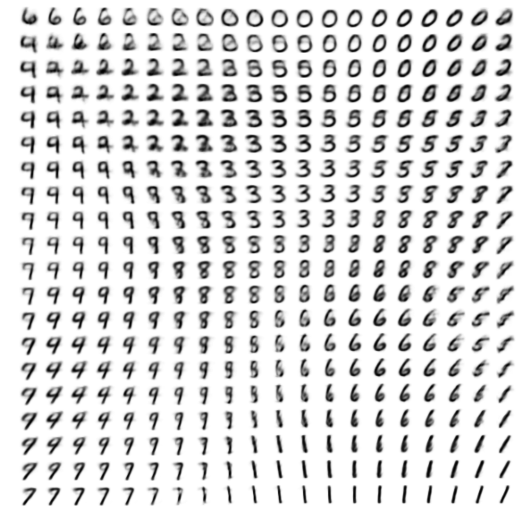
Each tile decodes one latent position. Follow a row or column to see digit shapes change. The paper obtains coordinates through Gaussian inverse-CDF mapping. This is a grid through a learned latent space, not a gallery of random independent samples; smooth changes do not prove disentangled concepts.

Kingma & Welling, Auto-Encoding Variational Bayes, Figure 4(b).

Failure Modes

• Posterior collapse: a strong decoder may ignore $z$, leaving $q_{\phi}(z\mid x)$ close to the prior.
• Approximation gap: the chosen variational family may poorly represent the true posterior.
• Likelihood mismatch: a convenient decoder distribution can produce undesirable sample or reconstruction behavior.
• Latent interpretation: smooth interpolation does not prove that latent coordinates correspond to independent human concepts.
• Anomaly detection: reconstruction or likelihood scores can fail on unfamiliar data and need task-specific validation.

The canonical source is Auto-Encoding Variational Bayes. Framework training code is intentionally omitted because the model assumptions and ELBO are the durable part.

My reading · Opened notes are remembered in this browser.