Recurrent Neural Networks

An RNN reuses parameters while carrying state through time:

$$\mathbf{h}_t=\phi(W_{xh}\mathbf{x}_t+W_{hh}\mathbf{h}_{t-1}+\mathbf{b}_h), \qquad \mathbf{o}_t=W_{ho}\mathbf{h}_t+\mathbf{b}_o.$$

The finite-dimensional state is a learned summary for the objective, not a lossless archive. That compression enables streaming and also loses long-range detail.

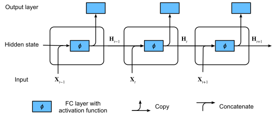Open full-size image

Read horizontally to follow the hidden state through time, then vertically to connect an input to its output. Repeated boxes represent repeated use of shared parameters, not separately trained networks. A later output can depend on earlier inputs through this state path.

Zhang et al., Dive into Deep Learning, recurrent neural network illustration. · CC BY-SA 4.0

Sequence Objectives

Form	Output	Example	Boundary
many-to-one	final or pooled state	sequence classification	can early evidence survive?
aligned many-to-many	every step	tagging, forecasting	masks and padding matter
autoregressive	next token/value	language, time series	train and generation inputs differ
encoder–decoder	conditional sequence	translation	one context can bottleneck history

Autoregressive modeling factorizes

$$p(x_{1:T})=\prod_{t=1}^{T}p(x_t\mid x_{<t}).$$

Teacher forcing supplies the true prefix in training; free generation uses the model's own earlier outputs, including their errors. Low teacher-forced loss therefore does not guarantee stable rollout. This difference is often called exposure bias. Its remedies depend on the task; longer training alone does not eliminate it.

Why Backpropagation Through Time Fails

The path from time $t$ to $k$ contains a Jacobian product:

$$\frac{\partial\mathbf{h}_t}{\partial\mathbf{h}_k} =\prod_{j=k+1}^{t}\operatorname{diag}(\phi'(\mathbf{z}_j))W_{hh}.$$

Repeated contraction causes vanishing gradients; expansion causes exploding gradients. Sequence length, weight spectra, activation saturation, and the trajectories encountered in the data all matter. The problem cannot be explained simply by calling RNNs old.

• Gradient clipping limits large updates but cannot restore vanished gradients.
• Truncated BPTT reduces memory and computation while truncating long-range credit assignment.
• Suitable initialization, normalization, and gates can improve training, without guaranteeing unlimited memory.

For clarity, define $J_j=\operatorname{diag}(\phi'(z_j))W_{hh}$. The ordered product is $J_tJ_{t-1}\cdots J_{k+1}$; matrix factors cannot generally be reversed. The same recurrent parameters appear at every step, so their gradient sums contributions from all uses, including indirect paths through later states. This is the chain-rule mechanism behind BPTT's gradient difficulties.

For the smoothing recurrence below with $\alpha=1/2$, $h_0=0$, and inputs $[2,0,4]$, states are $[1,0.5,2.25]$. The sensitivity to $h_0$ after three steps is $\alpha^3=1/8$. Detaching the state after step two preserves its numerical value $0.5$ for the next forward step but removes the gradient path to the earlier chunk. Detaching is not resetting. For padded sequences, masking only the loss is insufficient if a final state is consumed: skip padded state updates or select the last valid state.

LSTM Gating

A long short-term memory network (LSTM) maintains a cell state $\mathbf c_t$ alongside the hidden state $\mathbf h_t$. The forget gate $\mathbf f_t$ scales the previous cell state, the input gate $\mathbf i_t$ scales the candidate update $\tilde{\mathbf c}_t$, and the output gate $\mathbf o_t$ controls how the cell state contributes to $\mathbf h_t$. Here $\sigma$ is the sigmoid function, $\odot$ means elementwise multiplication, and $[\mathbf h_{t-1},\mathbf x_t]$ concatenates the two vectors. In these equations, $\mathbf o_t$ denotes the output gate, not the output scores in the opening RNN equation. A common form is:

$$\mathbf{f}_t=\sigma(W_f[\mathbf{h}_{t-1},\mathbf{x}_t]+\mathbf{b}_f), \quad \mathbf{i}_t=\sigma(W_i[\mathbf{h}_{t-1},\mathbf{x}_t]+\mathbf{b}_i),$$ $$\tilde{\mathbf{c}}_t=\tanh(W_c[\mathbf{h}_{t-1},\mathbf{x}_t]+\mathbf{b}_c), \quad \mathbf{c}_t=\mathbf{f}_t\odot\mathbf{c}_{t-1}+\mathbf{i}_t\odot\tilde{\mathbf{c}}_t,$$ $$\mathbf{o}_t=\sigma(W_o[\mathbf{h}_{t-1},\mathbf{x}_t]+\mathbf{b}_o), \quad \mathbf{h}_t=\mathbf{o}_t\odot\tanh(\mathbf{c}_t).$$

The additive cell path improves information and gradient flow. Gates are learned soft controls, not automatically interpretable memory switches; implementations vary in biases, projections, peepholes, and gate order.

Worked Example: Streaming Smoothing

Consider the scalar recurrence

$$h_t=\alpha h_{t-1}+(1-\alpha)x_t, \qquad 0<\alpha<1.$$

This is an exponential moving average. Each update uses constant memory. The newest observation has weight $1-\alpha$, and an observation $m$ steps old has weight $(1-\alpha)\alpha^m$.

The example shows both sides of recurrence: an RNN can update online without storing the whole sequence, but early information decays according to a fixed rule, and one old value cannot be reread on demand. A learned RNN is more flexible, yet remains constrained by its finite state and training signal. Attention changes this trade-off by retaining multiple represented positions and accessing them by content.

State and Data Boundaries

• Causal RNNs use only current and past inputs, so they support streaming prediction.
• Bidirectional RNNs also use future context, so they do not suit online decisions where that context is unavailable.
• Mask padding within a batch; sequence lengths revealed by padding must not leak labels.
• Reset hidden state between independent entities unless carrying it across the boundary has explicit meaning.
• Randomly splitting time-series windows can put adjacent or overlapping segments in both training and test.

The final item is data leakage rather than an architectural performance result. Design splits by entity and time.

Modern State-Based Sequence Models

Classical RNNs are not the end of state-based modeling. Structured state-space models (SSMs) start from continuous- or discrete-time linear state equations and use structured parameters and parallel algorithms to combine long-sequence training with recurrent inference. S4 demonstrated the long-sequence capabilities of structured SSMs; Mamba made parts of the update input-dependent and introduced a hardware-aware scan; xLSTM revisited recurrent memory and gates.

These names describe distinct architectures:

• A classical RNN's nonlinear state transition differs from an SSM's structured state equations.
• Mamba's linear sequence-scaling claim describes an algorithmic path, not guaranteed wall-clock superiority over attention at every length, batch size, or device.
• xLSTM continues the gated recurrent approach; it does not establish that LSTMs universally beat Transformers.
• Paper benchmarks remain tied to data, scale, kernels, and training budgets, and need replication on the target task.

As of 2026-08-11, S4, Mamba, and xLSTM are important competing designs, not a new permanent default.

RNNs, SSMs, and Full Self-Attention

Dimension	Classical RNN / some SSMs	Full self-attention
training path	RNN serial; structured SSMs may use parallel scans or convolutions	positions parallel within a layer
inference state	fixed or controlled size	KV cache usually grows with context
history access	compressed state	direct access to represented positions
long-range cost	state dynamics and selection	scores usually quadratic in length
useful counterexample	streaming sensors, low-memory settings, long sequences	large-scale parallel training and flexible content retrieval

Neither “Transformers made RNNs useless” nor “linear-time SSMs must replace attention” is justified. The choice depends on latency, memory, sequence length, training scale, kernels, and task structure.

Minimal Experiment

1. Overfit a short sequence to check the implementation.
2. Test whether changing masked padding leaves outputs unchanged.
3. Deliberately mix state boundaries and check that the tests catch the contamination.
4. Report teacher-forced loss and free-running results separately.
5. Split by time and entity, and compare with stateless, seasonal, or moving-average baselines.
6. Record gradient norms, truncation length, hidden width, kernels, and failed seeds.

This note favors supervised discrete sequences. Continuous-time systems, all SSM variants, reinforcement learning, and online feedback require separate treatment.

In Distill’s Visualizing memorization in RNNs, select characters in the autocomplete examples and inspect their connections to earlier input. Compare GRU and LSTM examples to see how similar aggregate scores can hide different uses of context. The displayed connections are gradient-based diagnostics for those examples, not a universal ranking of recurrent architectures.

My reading · Opened notes are remembered in this browser.