Convolutional Neural Networks

Convolutional neural networks (CNNs) encode two useful assumptions for grid-like data:

• locality: nearby values interact before distant values;
• parameter sharing: the same learned detector is applied across positions.

These assumptions reduce parameter count and make the representation translation equivariant: shifting the input tends to shift the resulting feature map. Equivariance is not the same as invariance. Pooling, aggregation, augmentation, and task design may produce some tolerance to shifts, but convolution alone does not make the output unchanged.

Cross-Correlation Layer

Deep-learning libraries usually implement cross-correlation even when the operation is called convolution. For input $\mathbf{X}$ and kernel $\mathbf{V}$,

$$H_{i,j,d} = b_d + \sum_a\sum_b\sum_c V_{a,b,c,d}\,X_{i+a,j+b,c}.$$

The kernel spans all input channels $c$ and produces one output channel $d$. Multiple learned kernels create multiple feature maps.

For one spatial dimension, kernel width $k$, padding $p$ on each side, and stride $s$, the output length is

$$\left\lfloor\frac{n+2p-k}{s}\right\rfloor+1.$$

The same calculation applies independently to height and width. Dilation adds spacing between kernel elements and changes the effective kernel size.

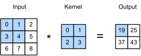Open full-size image

The shaded window uses the same kernel entries at every position. Its first output is 0×0 + 1×1 + 3×2 + 4×3 = 19. Sliding the window produces the remaining outputs. This is a single-channel, stride-one example without padding.

Zhang et al., Dive into Deep Learning, Figure 7.2.1. · CC BY-SA 4.0

Compute a Kernel and a Shape

For input $[1,2,4,8]$, kernel $[1,-1]$, zero bias, no padding, and stride one, cross-correlation produces $[-1,-2,-4]$: each output subtracts adjacent values. Mathematical convolution reverses the kernel and would produce $[1,2,4]$ under the same valid-window convention.

For an ordinary dense 2-D layer, input [B, 3, 32, 32] and 16 kernels of shape [3, 3, 3] (input channels, height, width), with padding one and stride two, give output [B, 16, 16, 16]. There are $16(3\cdot3\cdot3+1)=448$ learned parameters including biases, independent of image width and height. The shared weight gradient sums contributions from every position and batch example that used that weight.

With dilation $r$, replace $k$ by $r(k-1)+1$ in the output-length formula. The displayed cross-correlation equation assumes stride one, dilation one, and valid indices; padding supplies additional boundary values. As the padding and stride discussion illustrates, boundary treatment matters. Exact translation equivariance holds on an infinite grid for stride-one convolution; finite padding breaks it at edges, and stride-two sampling generally preserves only shifts aligned with the sampling grid. Pooling does not guarantee invariance to arbitrary shifts.

Building Blocks

• Padding controls border treatment and often preserves spatial size.
• Stride subsamples while applying the kernel.
• Pooling summarizes local neighborhoods without learned spatial weights.
• $1\times1$ convolution mixes channels independently at each spatial position.
• Stacked layers increase the receptive field and compose local features into higher-level representations.

Boundaries

• The useful inductive bias depends on the data; locality and translation structure are not universal.
• Downsampling can discard small or precisely located signals.
• A large receptive field does not prove that the model effectively uses all relevant context.
• Accuracy under random crops does not establish robustness to real distribution shift.
• Dataset construction and augmentation choices can dominate architecture changes.

Use a small MLP or linear model as a baseline when the input does not clearly benefit from spatial structure. For maintained implementations and exercises, see Dive into Deep Learning: Convolutional Neural Networks.

CNN Explainer lets you follow an example image through a small convolutional network. Inspect a convolution and its activation map, then compare what remains after pooling. This connects the local kernel calculation above to the changing spatial size and channel count across a full network.

My reading · Opened notes are remembered in this browser.