Transformers: Original Architecture and Modern Blocks

A Transformer is not synonymous with attention. It combines token representations, position, attention, feed-forward sublayers, residual paths, and normalization. The 2017 paper specified an encoder–decoder; common decoder-only blocks have since changed many details.

This page focuses on assembling a Transformer block, tensor shapes, and computational cost. Tokenization develops the full input pipeline; encoder, decoder, and encoder–decoder families explains context visibility and output heads; autoregressive decoding covers turning vocabulary scores into answers.

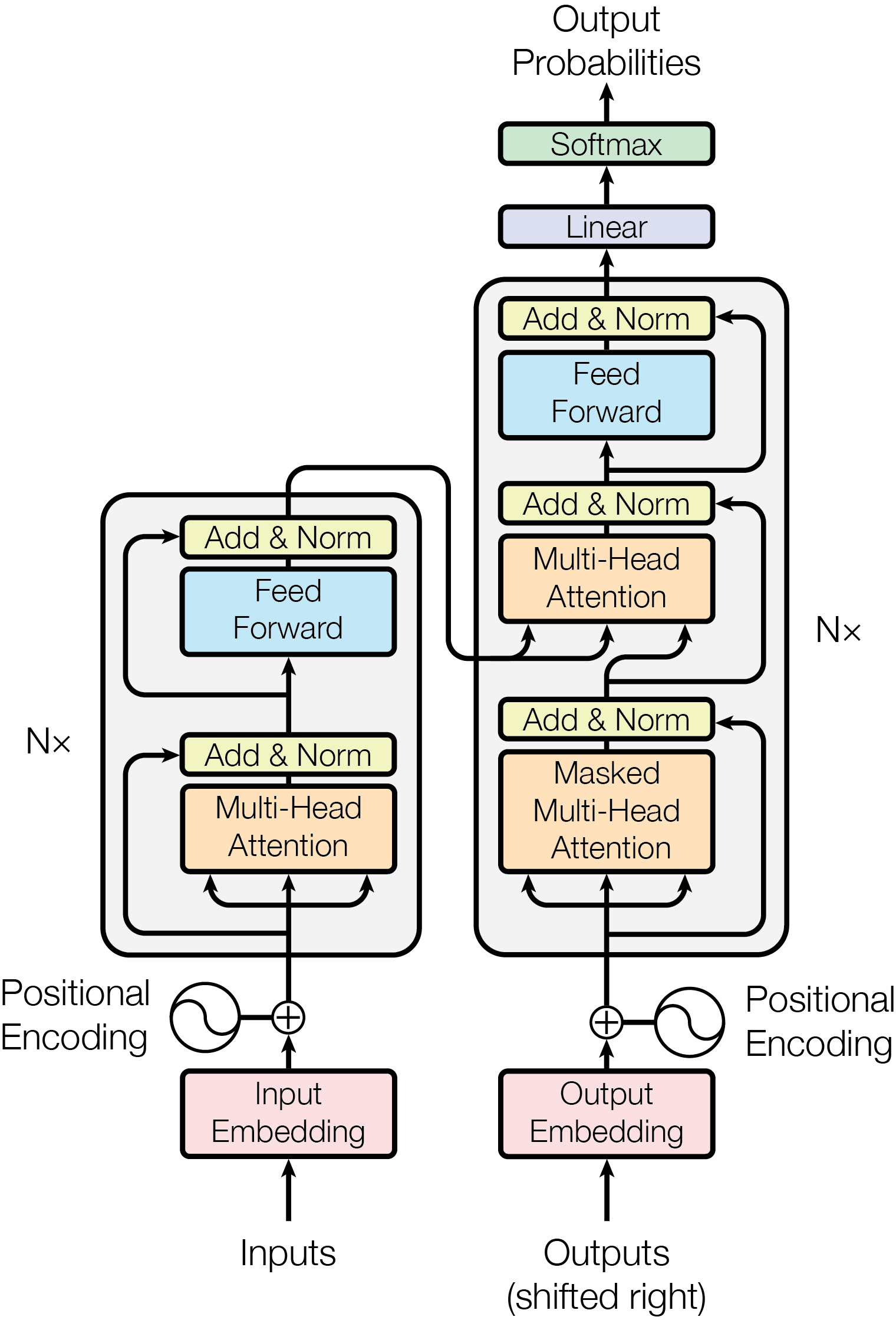Open full-size image

Read from the embeddings upward. The left stack encodes the input; the right stack uses earlier output tokens and the encoder’s representations. The arrows around each sublayer are residual connections. This is the original encoder–decoder with post-norm ordering; the pre-norm and decoder-only variants discussed below differ from this diagram.

Vaswani et al., Attention Is All You Need (2017), Figure 1. © Google. · Figure reuse permission

From Text to Input Vectors

A tokenizer converts text into vocabulary items and their integer token IDs. A token may be a word, part of a word, punctuation, or a byte-level unit; token boundaries and IDs depend on the tokenizer, not just the language. Special tokens can mark sequence boundaries or message roles.

For a toy vocabulary only, suppose BOS=0, hello=1, and world=2. The token sequence [BOS, hello, world] becomes IDs [0,1,2]. A learned embedding table $E\in\mathbb R^{|\mathcal V|\times d}$ supplies rows $E_0,E_1,E_2$, producing a $3\times d$ matrix, or shape [1,3,d] after adding a batch axis. IDs are lookup indices, not numerical measurements: ID 2 is not twice the meaning of ID 1. The original Transformer, §3.4, describes the learned input embeddings.

Position is incorporated according to the architecture below; the stack then makes these vectors context-dependent. An input token embedding is not automatically a sentence or document embedding suitable for retrieval. The vocabulary output projection in the training section closes the path from text to vectors and back to tokens.

Core Tensors

For $X\in\mathbb{R}^{b\times n\times d}$, learned projections produce Q/K/V. With $h_q$ query heads and $d_h=d/h_q$, common shapes are:

Q: [batch, h_q, sequence, d_h]
K: [batch, h_kv, sequence, d_h]
V: [batch, h_kv, sequence, d_h]

$$\operatorname{Attention}(Q,K,V)=\operatorname{softmax}\!\left(\frac{QK^{\top}}{\sqrt{d_h}}+M\right)V.$$

Multi-head attention (MHA) has $h_q=h_{kv}$; multi-query attention (MQA) uses $h_{kv}=1$; intermediate grouped-query attention (GQA) uses $1<h_{kv}<h_q$. The GQA paper also includes MHA and MQA as endpoint cases. MQA/GQA primarily reduce KV-cache traffic, not query count, and do not guarantee unchanged quality.

The attention formula must be applied with matching heads, not by blindly multiplying the displayed Q and K tensors. For equal-sized contiguous groups, require $h_q$ divisible by $h_{kv}$ and put $r=h_q/h_{kv}$. Zero-based query head $i$ shares KV head $g(i)=\lfloor i/r\rfloor$:

$$O_i=\operatorname{softmax}\!\left(\frac{Q_iK_{g(i)}^T}{\sqrt{d_h}}+M\right)V_{g(i)}.$$

With eight query heads and two KV heads, queries 0–3 use KV head 0 and queries 4–7 use KV head 1. Each output has shape [batch, sequence, d_h]; concatenating eight outputs restores width $d$. Explicitly repeating K/V across their query groups illustrates the semantics, but efficient kernels can share them without materializing those copies.

A Block Is More Than Attention

A plain FFN is

$$\operatorname{FFN}(x)=W_2\phi(W_1x+b_1)+b_2.$$

Modern blocks often use SwiGLU or GEGLU, with separate gate and value projections. FFNs often account for most of a block's parameters and compute.

Residual/norm order also varies:

• original Post-Norm: $y=\operatorname{LN}(x+\operatorname{Sublayer}(x))$;
• common Pre-Norm: $y=x+\operatorname{Sublayer}(\operatorname{Norm}(x))$.

Pre-Norm often makes deep-network training more stable, but is not mathematically equivalent to Post-Norm. LayerNorm centers and rescales variance; RMSNorm rescales by root mean square. Record epsilon, Pre/Post placement, and whether bias is included, rather than only saying “norm.”

What Is Normalized?

In a conventional Transformer, LayerNorm operates over the $d$ features of each token independently, not over batch or sequence positions. For one token $x$, it computes $\gamma\odot(x-\mu)/\sqrt{v+\epsilon}+\beta$, where $\mu=d^{-1}\sum_i x_i$ and $v=d^{-1}\sum_i(x_i-\mu)^2$. RMSNorm instead computes $\gamma\odot x/\sqrt{d^{-1}\sum_i x_i^2+\epsilon}$ in its usual bias-free form. For $x=[1,3]$, unit scale, zero bias and ignoring epsilon for this arithmetic example, LayerNorm gives $[-1,1]$, while RMSNorm gives $[1,3]/\sqrt5$. Neither uses BatchNorm-style running batch statistics; these normalization calculations stay the same at training and inference.

The FFN applies the same weights separately at each token position; attention is what mixes positions. The head outputs are concatenated and passed through a learned output projection back to width $d$, so the residual addition has matching shapes.

Position

Without positional information or an order-dependent mask, self-attention is permutation-equivariant: permuting input rows permutes output rows. A fixed causal mask already introduces order, so this unrestricted symmetry does not apply to it.

Method	Where it acts	Boundary
absolute position vector	added to token representation	extrapolation and length limits depend on the implementation
relative bias	modifies attention score	tied to bias form/window
RoPE	rotates pairs of coordinates in Q and K so dot products carry relative position	base, scaling, and extrapolation must be stated
ALiBi-like bias	distance-dependent score bias	a particular inductive bias, not universally best

RoPE is common in modern decoders. A configured long window does not prove effective retrieval, and position scaling may trade short-context quality.

Original Versus Common Modern Instances

Component	Original Transformer (2017)	Some modern decoder-only instances
topology	encoder–decoder	causal decoder stack
norm	Post-LayerNorm	Pre-RMSNorm or Pre-LayerNorm
position	sinusoidal absolute	RoPE or relative bias
FFN	ReLU	GELU, SwiGLU/GEGLU, sometimes MoE
heads	MHA	MHA, MQA, or GQA
kernel	conventional matrices	fused SDPA, FlashAttention

The right column is not one standard. Llama 3's RMSNorm, RoPE, GQA, and SwiGLU form one documented package; it neither defines every Transformer nor isolates one component's contribution.

Worked Shape and Memory Estimate

For batch=2, $n=128$, $d=512$, and $h=8$, $d_h=64$:

Q/K/V: [2, 8, 128, 64]
attention scores: [2, 8, 128, 128]
concatenated output: [2, 128, 512]

For batch=1, $n=4096$, and eight heads, scores contain

$$8\times4096^2=134{,}217{,}728$$

elements. At fp16, the score matrix alone occupies about 256 MiB, before gradients, Softmax intermediates, Q/K/V projections, FFNs, and additional layers. FlashAttention uses tiling to avoid materializing the whole intermediate matrix and reduce peak memory, but exact full-attention arithmetic remains quadratic.

Training and Generation Are Different Systems

Causal-LM training computes positions in parallel for a known sequence; generation depends token by token on prior outputs. KV caching avoids recomputing old K/V, but its main storage is proportional to the product of layer count, context length, K/V-head count, head dimension, batch size, and bytes per element.

Performance reports should distinguish:

• Prefill latency from decode latency.
• Throughput at specified batch sizes, prompt/output lengths, and sampling settings.
• Cache quantization, windowing, paging, or offload strategies.
• Training activation memory from inference resident memory.
• Kernel implementation, compiler, hardware, and precision.

“1M context” or “uses FlashAttention” does not establish end-to-end usability.

The stack outputs a hidden vector $h_t\in\mathbb R^d$ at each position, not a token ID. A vocabulary projection $W_{\mathrm{vocab}}\in\mathbb R^{d\times|\mathcal V|}$ produces logits $z_t=W_{\mathrm{vocab}}^Th_t+b$. Softmax and cross-entropy turn these scores into a distribution over vocabulary items and a training loss against the next-token target. Generation selects or samples from that distribution; its normalized axis is vocabulary items, whereas attention normalizes over keys.

For a concrete next-token training example, use inputs [BOS, A, B] and targets [A, B, EOS]. Each input position sees itself and earlier inputs only; feeding unshifted targets leaks the answer even with a causal mask. The 2017 encoder–decoder adds cross-attention between masked decoder self-attention and the FFN: decoder states supply queries, encoder outputs supply keys and values, and all valid source positions are visible. Source padding is still masked.

At generation time, process the prompt once (prefill), use its last output to select the next token, then feed that token through the stack (decode). With an exact cache and unchanged causal prefix, old states cannot depend on the appended token, so their K/V remain reusable. Dropout must be disabled for deterministic cached-versus-uncached comparisons. Cache size and reuse conditions are developed in Attention Variants and KV-Cache Compression.

Architecture Families

• Encoder-only: Uses bidirectional context, often for representation learning or discriminative tasks.
• Decoder-only: Uses causal objectives and suits generation tasks.
• Encoder–decoder: Separates input encoding from conditional generation and suits sequence-transformation tasks.
• MoE Transformer: Routes tokens through a subset of experts, increasing total capacity while introducing load-balancing needs, communication overhead, and routing-failure risks.

These labels remain insufficient for reproduction: tokenizer, data, objective, context curriculum, optimizer, post-training, and tool protocol often affect final behavior more than an individual block detail.

For expert selection, load balancing, and the difference between total and active parameters, see Mixture of Experts.

Failure Modes and Counterexamples

• A reversed causal mask leaks future tokens.
• Padding, packing, or cross-document attention can contaminate training.
• Long contexts may use information in the middle less effectively than information at the beginning or end.
• Architecture changes do not repair benchmark or corpus contamination.
• RoPE scaling, GQA, quantization, and fused kernels can interact and degrade performance at particular lengths or dtypes.
• Fixed-memory streaming may favor RNNs/SSMs over a growing KV cache.
• In local vision tasks, convolution's inductive bias may need less data than attention.

Minimal Reproduction Configuration Card

architecture: encoder | decoder | encoder-decoder
layers: N
width: d_model
attention: heads, kv_heads, head_dim, window, kernel
position: method, base, scaling, trained_length
norm: type, pre_or_post, epsilon
ffn: activation_or_gate, intermediate_width, experts
training: objective, data boundary, precision, optimizer, seeds
inference: cache, quantization, batch, prompt/output lengths

Current products and APIs belong in the Frontier Radar; this page maintains reusable architectural boundaries.

In Transformer Explainer, enter a short prompt and follow its tokens through attention, the MLP, and next-token probabilities. Change temperature while keeping the prompt fixed to separate the model’s logits from the sampling decision. The demonstration uses GPT-2, so compare its decoder-only blocks with the original encoder–decoder diagram above.

My reading · Opened notes are remembered in this browser.