Attention Variants and KV-Cache Compression

During autoregressive decoding, each new token attends to keys and values from earlier tokens. Caching those tensors avoids recomputing them, but cache memory grows linearly with sequence length and batch size. Reading the cache can become a major bandwidth cost, especially for long contexts and small decode batches.

The main approaches reduce one of three things: the number of KV heads, the width of the cached representation, or the number/precision of cached tokens.

Open full-size image

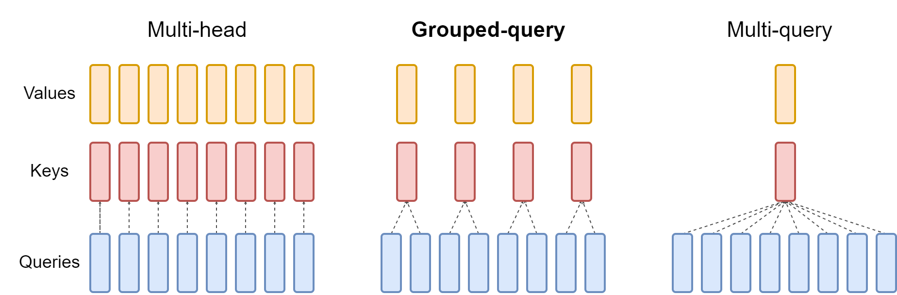
Read upward from the blue query heads. In the middle, each pair of queries shares one key/value pair; on the right, all queries share one pair. The query count stays fixed. The cache saving comes from storing fewer keys and values, with other dimensions held constant.

Ainslie et al., GQA (2023), Figure 2. · CC BY 4.0

MHA and GQA

Let a model have $L$ layers, sequence length $S$, $n_h$ query heads, $n_{kv}$ KV heads, head dimension $d_h$, and $b$ bytes per cached element. Ignoring allocator and metadata overhead, the KV cache for one sequence is approximately

$$2L S n_{kv} d_h b.$$

The factor of two accounts for keys and values.

• Multi-head attention (MHA) normally uses $n_{kv}=n_h$.
• Multi-query attention (MQA) uses one KV head shared by all query heads.
• Grouped-query attention (GQA) lies between them: several query heads share each KV head.

Holding the other dimensions fixed, changing from MHA to GQA reduces this part of cache memory in proportion to $n_{kv}/n_h$. Whether quality, throughput, and kernel support remain acceptable depends on the trained model and serving stack; GQA is an architectural choice made during training, not a lossless switch applied to arbitrary weights.

For a hypothetical $L=32$, $S=4096$, $n_h=32$, $n_{kv}=8$, $d_h=128$, and two-byte elements, this is $536{,}870{,}912$ bytes, or 512 MiB per sequence. MHA with 32 KV heads would use 2 GiB; four equal-length GQA sequences use 2 GiB before overhead. These are cache estimates, not total model-memory estimates.

When Is Reuse Exact?

For a causal model in evaluation mode, appending a token does not change previous token representations. Each layer caches its own K/V; queries are recomputed only for the new positions. Exact reuse requires the same tokenized prefix, weights (including adapters), position indices, attention rules, and numerical representation. Editing an earlier token invalidates downstream cached states. Bidirectional attention generally cannot reuse old states unchanged after appending input, since those states may attend to the new token.

With $S$ cached tokens and a new chunk of $q$ tokens, query row $i$ (zero-based within the chunk) may attend through absolute key position $S+i$. A naive $q\times(S+q)$ upper-left triangular mask would hide valid cached keys. Preserve original position indices after eviction; renumbering retained tokens changes positional attention. Test cached against uncached logits on the same prefix before testing approximate compression, allowing for floating-point differences from changed kernel shapes or reduction order.

Tree speculation extends this state-management problem to candidate branches: isolate them and retain KV and compressed states along the accepted path.

Multi-head latent attention

DeepSeek-V2 introduced multi-head latent attention (MLA). Instead of caching full per-head key and value tensors, the model learns a lower-dimensional latent representation. Parts of the key path used for rotary position information remain separate because the position-dependent rotation cannot simply be folded into a fixed projection.

A simplified cache-width comparison is:

$$\begin{aligned} \text{MHA/GQA width per token per layer} &\approx 2n_{kv}d_h,\\ \text{MLA width per token per layer} &\approx d_c+d_R, \end{aligned}$$

where $d_c$ is the compressed latent width and $d_R$ is the decoupled rotary-key width. The actual memory and compute path depends on the model's exact projections and the inference implementation. MLA can greatly reduce cache traffic, but its published results belong to models trained with that architecture.

Compressing an existing cache

Methods such as SnapKV and PyramidKV operate on the tokens retained in an existing model's cache rather than changing the trained attention architecture.

• SnapKV scores prompt positions using attention patterns from an observation window and retains a selected subset of past keys and values.
• PyramidKV gives different layers different cache budgets, motivated by observed differences in how layers distribute attention over the prompt.
• KV-cache quantization stores cache elements at lower precision.
• Windowed or sliding attention keeps only a bounded recent region in layers designed to support it.

These techniques are not interchangeable. Token eviction can lose a small but decisive passage; quantization can change attention scores; custom layouts may need specialized kernels. Paper-level accuracy or perplexity results apply to the evaluated models, tasks, budgets, and implementations—not to every long-context workload.

What to measure

For a concrete deployment, record:

1. exact model, attention architecture, and cache dtype;
2. prompt length, generated length, and concurrent sequences;
3. peak GPU and host memory;
4. prefill time, time to first token, and decode throughput;
5. task success on long-context cases that require information from different positions;
6. the behavior after cache eviction, quantization, or CPU offload.

A model that advertises a long context window may still be unusable on the available hardware, while a cache-saving method that fits may still fail the task. Memory fit and retained answer quality need separate tests.

My reading · Opened notes are remembered in this browser.