Automatic Differentiation

PyTorch Autograd Explained - In-depth Tutorial - YouTube 2.5. Automatic Differentiation — Dive into Deep Learning documentation

Automatic Differentiation in JAX

JAX is a library for high-performance numerical and scientific computing on modern hardware, including GPUs and TPUs. It extends NumPy with automatic differentiation and uses function transformations to compute gradients efficiently. These gradients are central to optimization problems and machine learning algorithms.

Automatic Differentiation (Autodiff)

Automatic differentiation evaluates derivatives by composing the derivative rules of elementary operations along a program's calculation, using the chain rule. Unlike symbolic differentiation, it need not build a simplified formula; unlike finite differences, it does not estimate a derivative from nearby function values. It differentiates the implemented computation, subject to floating-point error and the available rules. A discontinuity, integer decision, unsupported operation, or undefined derivative is not made differentiable by autodiff. Higher derivatives require sufficient differentiability and can be expensive. Review derivatives and the matrix shapes of linear maps before Jacobian products.

Forward and Reverse Mode Autodiff

For $f:\mathbb R^n\to\mathbb R^m$, the Jacobian $J$ has entries $J_{ij}=\partial f_i/\partial x_j$ and shape $m\times n$. Forward mode propagates an input direction $v\in\mathbb R^n$ to $Jv\in\mathbb R^m$. Reverse mode propagates output weights $u\in\mathbb R^m$ to $J^Tu\in\mathbb R^n$. Basis-vector seeds recover individual columns or rows; neither mode is limited to a single coordinate seed.

The transpose comes from the multivariable chain rule, not a convention of JAX. Let $z=f(x)$ and let $L(z)$ be a scalar loss. Each input can affect the loss through every output, so

$$\frac{\partial L}{\partial x_j}=\sum_i\frac{\partial L}{\partial z_i}\frac{\partial z_i}{\partial x_j}, \qquad \nabla_xL=J^T\nabla_zL.$$

Thus reverse mode uses $u=\nabla_zL$. The sum is also why contributions from separate paths must accumulate. This is the scalar chain rule applied to all intermediate coordinates.

A full Jacobian therefore takes roughly $n$ forward sweeps or $m$ reverse sweeps. Forward mode suits few inputs and many outputs; reverse mode suits many inputs and few outputs, especially a scalar loss. Reverse mode underlies backpropagation, but must retain or recompute intermediates for the backward sweep. These are work/memory trade-offs, not a universal speed ranking.

Differentiation Graph

A differentiation graph is a graphical representation of a function's computation, recording each operation from input to output, its intermediate variables, and their dependencies.

Automatic differentiation uses this graph to apply the chain rule efficiently and accurately:

• In forward mode, derivatives propagate in the direction of the graph.
• In reverse mode, gradients accumulate in the opposite direction.

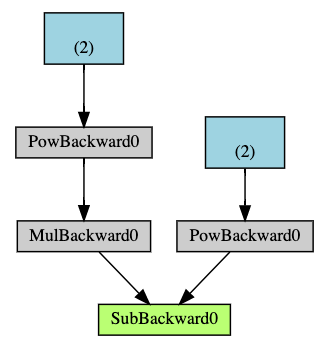Open full-size image

This PyTorch example computes Q = 3a³ − b² elementwise. Read downward to follow the forward calculation and upward to trace gradient propagation. Labels such as PowBackward0 name the stored backward functions; “(2)” is the input tensor’s shape. The JAX code below uses a different function, but likewise combines elementary derivative rules to obtain the result.

PyTorch contributors, A Gentle Introduction to torch.autograd. · BSD 3-Clause

How JAX Implements Autodiff

JAX supports both forward and reverse mode to compute gradients, Jacobians, and Hessians efficiently. Its main interfaces are:

• jax.grad:

  • Computes a function's gradient.
  • Uses reverse mode.
  • Suits cases with far more input dimensions than output dimensions, such as a neural network's scalar loss.

• jax.jvp (Jacobian-vector product):

  • Computes a Jacobian-vector product.
  • Is the basic forward-mode operation.
  • Computes $J \cdot v$, where $J$ is the Jacobian and $v$ is a vector.

• jax.vjp (vector-Jacobian product):

  • Computes a vector-Jacobian product.
  • Is the basic reverse-mode operation.
  • Computes $v^T \cdot J$, where $v$ is a vector and $J$ is the Jacobian.

Example Usage

This example uses JAX to compute a function's gradient:

import jax
import jax.numpy as jnp

def f(x):
    return jnp.sin(x) * jnp.cos(x)

# Obtain the gradient function of f
grad_f = jax.grad(f)

# Compute the gradient of f at x = 1.0
print(grad_f(1.0))

This code snippet computes the derivative of the function $f(x) = \sin(x) \cos(x)$ at the point $x = 1.0$.

Work through a shared input

Let $a=xy$, $b=\sin x$, and $f=a+b$. At $(x,y)=(2,3)$, a forward seed $(\dot x,\dot y)=(1,0)$ gives $\dot a=y\dot x+x\dot y=3$ and $\dot b=\cos2$, so $\dot f=3+\cos2\approx2.583853$. This is $J(1,0)^T$.

For reverse mode, seed $\bar f=1$. Addition sends $\bar a=\bar b=1$. The multiplication contributes $y\bar a=3$ to $\bar x$ and $x\bar a=2$ to $\bar y$; sine contributes $\cos2\,\bar b$ to $\bar x$. Contributions to the same input must be added, giving $\nabla f=(3+\cos2,2)$. The two routes through $x$ are why simply overwriting its gradient is wrong.

In the earlier JAX example, the expected derivative is $\cos^2(1)-\sin^2(1)=\cos2\approx-0.416147$. jax.grad expects a scalar output (shape (), not a length-one vector) and ordinarily differentiates floating-point inputs. For vector outputs, choose jax.jvp, jax.vjp, jax.jacfwd, or jax.jacrev according to the product or matrix needed. At a kink such as $|x|$ at zero, an implementation's chosen rule is not proof that a classical derivative exists.

References and Useful Links

• The Autodiff Cookbook — JAX documentation
• Automatic Differentiation Videolectures

My reading · Opened notes are remembered in this browser.