Softmax Regression

Softmax regression is a linear model that assigns probabilities to $K$ mutually exclusive classes, commonly used for single-label classification. It produces one unnormalized score, or logit, per class:

$$\mathbf{o} = \mathbf{W}^{\top}\mathbf{x} + \mathbf{b}.$$

Follow one example with three classes and logits $[\log 2,0,0]$. Exponentiating gives $[2,1,1]$, whose sum is $4$. Dividing each entry by $4$ gives probabilities $[1/2,1/4,1/4]$.

Softmax converts the logits into nonnegative values that sum to one:

$$p(y=k\mid\mathbf{x}) = \frac{\exp(o_k)}{\sum_{j=1}^{K}\exp(o_j)}.$$

Implementations subtract the largest logit before exponentiation for numerical stability; this does not change the result because softmax is invariant to adding the same constant to every logit. At inference, argmax can operate directly on logits because softmax preserves their ordering.

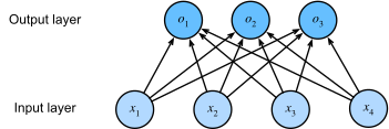Open full-size image

Each output combines all four inputs using its own weights and bias. The three output nodes are logits, not probabilities: softmax normalizes them afterward. There is no hidden layer. With the matrix convention above, this example has W of shape 4 × 3 and three bias terms.

Zhang et al., Dive into Deep Learning, Figure 4.1.1. · CC BY-SA 4.0

Cross-Entropy

For a one-hot target $\mathbf{y}$, the per-example cross-entropy is (with $p_y$ denoting the probability assigned to the observed class)

$$\ell(\mathbf{y},\mathbf{p}) = -\sum_{k=1}^{K} y_k\log p_k = -\log p_{y}.$$

Suppose the second class is correct, so the one-hot target is $\mathbf y=[0,1,0]$. Only its probability contributes: $\ell=-\log(1/4)=\log4\approx1.3863$. The model favors the first class, but raising the second class’s probability would reduce this loss.

Minimizing this objective corresponds to maximizing the conditional likelihood of the observed class labels under the model.

The information-theory definition of cross-entropy compares a target distribution with a predictive distribution. Here the one-hot $\mathbf y$ is the empirical target for one observed example, and $\mathbf p$ is the prediction. Natural logarithms give loss in nats. This does not imply that the population's conditional label distribution is itself one-hot.

A Stable Loss and Its Gradient

For $d$ input features, $W$ is $d\times K$, $b$ is length $K$, and a batch of $B$ rows produces $B\times K$ logits. Let $c$ be the correct class index, distinct from the one-hot vector $y$. The softmax derivation yields

$$\ell= m+\log\sum_j e^{o_j-m}-o_c, \quad m=\max_j o_j, \qquad \frac{\partial\ell}{\partial o_j}=p_j-y_j.$$

Compute this log-sum-exp expression or use a fused cross-entropy loss that accepts logits. Taking a logarithm of already rounded probabilities can produce infinity even after stable softmax.

In the same example, $m=\log2$ and $o_c=0$, so the stable loss is $\log2+\log(1+1/2+1/2)-0=\log4$. Adding $1000$ to every logit cancels out of this expression and leaves both loss and probabilities unchanged.

Subtract the target from the prediction to find the direction of correction:

$$\mathbf p-\mathbf y=[1/2,1/4,1/4]-[0,1,0]=[1/2,-3/4,1/4].$$

The negative second component calls for raising the correct logit; the positive components call for lowering the others. A gradient-descent step on these logits subtracts a positive multiple of this vector.

To connect the logits to the trainable parameters, differentiate $\ell=\log\sum_k e^{o_k}-o_c$ and use $o_j=\sum_i W_{ij}x_i+b_j$:

$$\frac{\partial\ell}{\partial o_j}=p_j-\mathbf1_{j=c},\qquad \frac{\partial\ell}{\partial W_{ij}}=x_i(p_j-y_j),\qquad \frac{\partial\ell}{\partial b_j}=p_j-y_j.$$

This is reverse-mode differentiation through the affine logits: the loss gradient is passed backward and scaled by the corresponding input. The matrix formula $\nabla_W\ell=x(p-y)^T$ collects those coordinate derivatives. A mean batch loss averages these per-example gradients.

Boundaries

• Mutually exclusive multiclass: softmax regression commonly models a single class label per example. The softmax function also serves other purposes, such as computing attention weights.
• Multilabel: use independent outputs, commonly sigmoid probabilities with a binary loss, when several labels may be true simultaneously.
• Decision rule: argmax chooses a class, but asymmetric costs may require a different rule.
• Probability quality: good classification accuracy does not imply calibrated probabilities.
• Linear boundary: nonlinear feature relationships require transformed features or a more expressive model.

Evaluate against class frequencies and a simple baseline, then inspect a confusion matrix and per-class errors. Aggregate accuracy can hide poor behavior on rare or important classes.

Continue with the Multilayer Perceptron to introduce nonlinear hidden representations. See Dive into Deep Learning: Linear Neural Networks for Classification for derivations and maintained implementations.

My reading · Opened notes are remembered in this browser.