Gradient and Multidimensional Optimization

Definition of Gradient

For a differentiable function $f(x, y)$ with two variables, using Euclidean coordinates, the gradient, denoted as $\nabla f$, is defined as the vector of its partial derivatives. Formally,

$$\nabla f = \left( \frac{\partial f}{\partial x}, \frac{\partial f}{\partial y} \right)$$

For $f(x, y) = x^2 + y^2$, the gradient is $\nabla f = (2x, 2y)$. This vector points in the direction of greatest local increase, and its magnitude gives that maximum directional rate of change. At a regular point, the gradient is perpendicular—not tangent—to the level curve through that point.

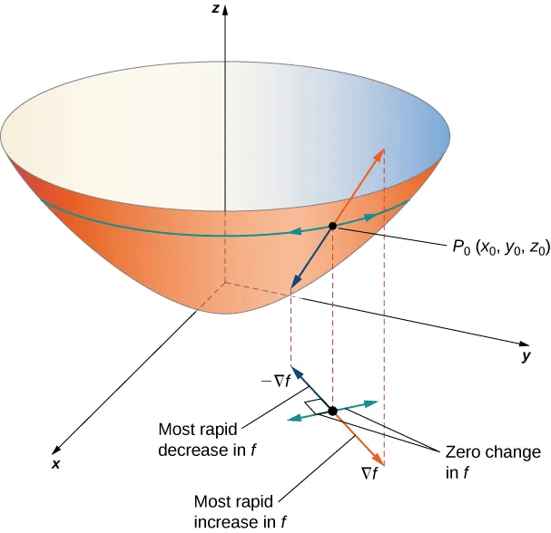Open full-size image

Start with the arrows in the lower plane: the gradient lives in the input coordinates (x, y). Orange points toward steepest local increase, blue toward decrease, and green is tangent to a level curve. The surface above shows the corresponding changes in height; the gradient itself is not a three-dimensional arrow on that surface.

Gilbert Strang & Edwin Herman, OpenStax, Calculus Volume 3, Figure 4.41. · CC BY-NC-SA 4.0

Gradient at a Specific Point

To find the gradient of $f(x, y) = x^2 + y^2$ at a particular point, say $(2, 3)$, we substitute $x = 2$ and $y = 3$ into the gradient formula:

$$\nabla f = (2 \cdot 2, 2 \cdot 3) = (4, 6)$$

This result signifies the gradient of $f$ at the point $(2, 3)$ and represents the vector pointing in the direction of greatest increase of $f$ from that point.

Why the negative gradient gives local descent

Assume $f$ is differentiable at an interior point $q$. For a unit vector $u$ in the Euclidean norm, the directional derivative is

$$D_u f(q)=\lim_{t\to0}\frac{f(q+tu)-f(q)}t=\nabla f(q)^Tu.$$

Cauchy–Schwarz gives $-\|\nabla f(q)\|_2\le D_u f(q)\le\|\nabla f(q)\|_2$. If the gradient is nonzero, the lower bound is attained at $u=-\nabla f(q)/\|\nabla f(q)\|_2$. This is steepest descent among Euclidean unit directions, not a promise about a long step or differently scaled coordinates. In particular,

$$f(q-\alpha\nabla f(q))=f(q)-\alpha\|\nabla f(q)\|_2^2+o(\alpha),$$

so sufficiently small positive steps decrease $f$. For the gradient $(4,6)$ above, the steepest unit direction is $(-2,-3)/\sqrt{13}$ and its rate is $-2\sqrt{13}$. A tangent vector $v$ to a regular level curve satisfies $\nabla f(q)^Tv=0$ by differentiating the constant value along that curve.

Hessian and directional curvature

For a twice continuously differentiable function, the Hessian collects second partial derivatives, $H_{ij}(q)=\partial^2 f(q)/\partial x_i\partial x_j$. Equality of mixed partials makes it symmetric. The second-order expansion is

$$f(q+v)=f(q)+\nabla f(q)^Tv+\tfrac12v^TH(q)v+o(\|v\|_2^2).$$

The quadratic form $v^THv$ describes curvature along a displacement. A real symmetric matrix is positive definite if this is positive for every nonzero $v$, and positive semidefinite if it is nonnegative. These correspond to all eigenvalues being positive or nonnegative, respectively. An indefinite matrix has directions with both signs. See Boyd and Vandenberghe, Appendix A and §3.1.4 for the matrix definitions and second-order convexity criterion.

For $x^2-y^2$, $H=\operatorname{diag}(2,-2)$: curvature is positive along the x-axis and negative along the y-axis. For a symmetric $2\times2$ matrix, positive definiteness is equivalent to $H_{11}>0$ and $\det H>0$, the test used in the regression example below. A zero Hessian is inconclusive: $x^4+y^4$, $-x^4-y^4$, and $x^4-y^4$ all have one at the origin but give a minimum, maximum, and saddle. Positive semidefiniteness throughout an open convex domain, rather than at one point, underlies the global guarantee in convex optimization.

A stationary point has zero gradient; a local minimum is best among nearby feasible points; a global minimum is best over the entire feasible set. These differ: $x^2-y^2$ has a stationary saddle at the origin, while minimizing $x$ on $[0,1]$ gives the boundary solution $0$ with derivative $1$. At a stationary point of a twice continuously differentiable function, a positive-definite Hessian ensures a strict local minimum; an indefinite Hessian gives a saddle, and a singular positive-semidefinite Hessian needs further analysis.

Application in Optimization

At an interior local extremum of a differentiable function, the derivative must vanish. The converse is not guaranteed. For $f(x)=x^2$, solving $f'(x)=2x=0$ gives the candidate $x=0$; the separate inequality $x^2\ge0$ proves it is the global minimum. Boundary points and points where a derivative does not exist require separate consideration.

For functions of two or more variables, such as $f(x, y) = x^2 + y^2$, the optimization process seeks points where the gradient is zero, i.e., $\nabla f = \vec{0}$. This condition implies that both partial derivatives, $\frac{\partial f}{\partial x}$ and $\frac{\partial f}{\partial y}$, are zero. Solving the system of equations

$$\begin{align*} \frac{\partial f}{\partial x} = 2x &= 0 \\ \frac{\partial f}{\partial y} = 2y &= 0 \end{align*}$$

yields the point $(0, 0)$ as the location of the minimum. This search generalizes to functions of any number of variables, but a zero gradient identifies only a stationary candidate. The point may be a minimum, maximum, or saddle, so a second-order test or another argument is still needed.

Optimization in a Two-Dimensional Sauna

Considering a sauna as a two-dimensional space allows for movement in any direction within a 5x5 room, aiming to find the coldest point based on the temperature distribution.

• Temperature Function: For a given position $(x, y)$, the temperature is a function $T(x, y)$ represented by the height in a three-dimensional plot. Hot areas are indicated by red (higher values) and cold areas by blue (lower values).

• Objective: Minimize $T(x,y)$ over the closed square $[0,5]^2$. A global minimizer need not be an interior point or have strictly higher values at every other point.

• Mathematical Approach: The process involves calculating the partial derivatives $\frac{\partial T}{\partial x}$ and $\frac{\partial T}{\partial y}$, setting them to zero, and solving for $x$ and $y$ to find potential minimum points.

• Example Function: $T(x, y) = 85 - \frac{1}{90}x^2(x - 6)y^2(y - 6)$.

• Partial Derivatives:

  $$\frac{\partial T}{\partial x} = -\frac{1}{90}x(3x - 12)y^2(y - 6)$$ $$\frac{\partial T}{\partial y} = -\frac{1}{90}x^2(x - 6)y(3y - 12)$$

• Finding the Minimum: Solving $\frac{\partial T}{\partial x}=0$ and $\frac{\partial T}{\partial y}=0$ gives interior candidates only. Check the four edges and corners as well; the complete argument below includes the boundary.

For the sauna, declare the domain $[0,5]^2$. Put $h(t)=t^2(6-t)$, so $T=85-h(x)h(y)/90$. On $[0,5]$, $h\ge0$ and $h'(t)=3t(4-t)$: it increases to $h(4)=32$ and then decreases. Thus the unique global coldest point is $(4,4)$ with $T=3313/45\approx73.6222$. Edges with $x=0$ or $y=0$ have temperature $85$; edges at $5$ have minimum $85-25\cdot32/90\approx76.1111$. This checks the boundary, not just stationary points.

Linear Regression Optimization

Linear regression, a fundamental machine learning model, is optimized through a similar multidimensional calculus approach but involves finding the best fit line to a set of data points.

• Problem Statement: With given coordinates of power lines, the task is to minimize the total cost of connecting these to a main fiber line. In this illustrative model, cost is proportional to squared vertical residuals, not shortest distances to the line.
• Mathematical Formulation: The line equation $y = mx + b$ represents the fiber line, with $m$ and $b$ being the slope and y-intercept, respectively. The optimization goal is to minimize the total cost function $E(m, b)$, which depends on $m$ and $b$.
• Cost Function: Use the illustrative data $(1,2),(2,5),(3,3)$. Expanding the vertical residual sum $E(m,b)=(m+b-2)^2+(2m+b-5)^2+(3m+b-3)^2$ gives $14m^2+3b^2+38+12mb-42m-20b$.
• Partial Derivatives and Optimization:
  • $\frac{\partial E}{\partial m} = 28m + 12b - 42$
  • $\frac{\partial E}{\partial b} = 6b + 12m - 20$
• Solution: Setting $\frac{\partial E}{\partial m} = 0$ and $\frac{\partial E}{\partial b} = 0$ and solving for $m$ and $b$ yields the optimal line parameters minimizing the cost.
• Result: The optimal values $m = \frac{1}{2}$ and $b = \frac{7}{3}$ are found, with a minimum cost of 4.167.

For the regression quadratic, the Hessian is $\begin{pmatrix}28&12\\12&6\end{pmatrix}$, with positive leading minor $28$ and determinant $24$. It is positive definite, so $(1/2,7/3)$ is the unique global minimizer and $E_{\min}=25/6\approx4.1667$. Here squared distance means a vertical residual $y_i-(mx_i+b)$; perpendicular distance would also divide its square by $1+m^2$ and give a different optimization problem. For the statistical model, see Linear Regression.

Gradient Descent: An Efficient Optimization Method

When solving stationary equations directly is impractical, gradient descent offers an iterative alternative. It is not always faster than a direct solver, and descent alone does not establish convergence or global optimality. The local descent property follows from differentiability as shown above; the one-variable guide supplies a domain-safe implementation.

My reading · Opened notes are remembered in this browser.