Linear Algebra

Linear algebra studies spaces and transformations that preserve addition and scaling. A durable learning sequence is:

1. vectors, span, independence, basis, and dimension;
2. linear maps and their matrix representations;
3. systems of equations, elimination, rank, and null spaces;
4. inner products, orthogonality, projections, and least squares;
5. determinants, eigenvalues, and eigenvectors;
6. singular value decomposition and low-rank approximation;
7. applications to optimization, data analysis, and machine learning.

The reference below covers finite-dimensional real vectors, linear systems, and least squares. It assumes elementary algebra; MIT OpenCourseWare 18.06SC develops the proofs and the later factorization topics in the sequence above.

Vectors, bases, and shapes

A vector in $\mathbb R^n$ has $n$ real coordinates relative to a chosen basis. The span of some vectors is the set of their linear combinations. They are linearly independent if the only combination giving zero has every coefficient zero. A basis is an independent spanning set; its size is the dimension. For example, $(1,0)$ and $(0,1)$ form a basis of $\mathbb R^2$, while $(1,2)$ and $(2,4)$ span only a line.

A linear map satisfies $T(au+bv)=aT(u)+bT(v)$. With column vectors, a matrix $A\in\mathbb R^{m\times n}$ maps an input $x\in\mathbb R^n$ to $Ax\in\mathbb R^m$. Its columns are the images of the input basis vectors. Thus $Ax$ is a weighted sum of columns. If $B\in\mathbb R^{n\times k}$, then $AB\in\mathbb R^{m\times k}$ applies $B$ first, then $A$; $BA$ may not even be defined. Adding a nonzero bias, $Ax+b$, gives an affine map, not a linear one.

Watch the basis vectors and grid move together in 3Blue1Brown’s lesson on linear transformations. Reading the images of the basis vectors as matrix columns gives a visual counterpart to the column-vector convention used here.

When does a system have a solution?

The column space of $A$ is the span of its columns: all vectors that can be written as $Ax$. The rank of $A$ is the dimension of that space. Its null space, written $\ker A$, consists of vectors $z$ with $Az=0$; $\dim$ denotes dimension. For a matrix with $n$ columns, rank–nullity gives $\dim\ker A=n-\operatorname{rank}(A)$. In the tests below, $[A\mid b]$ means the matrix formed by appending $b$ as an extra column.

• $Ax=b$ is solvable exactly when $b$ lies in the column space, equivalently $\operatorname{rank}(A)=\operatorname{rank}([A\mid b])$.
• If $x_0$ is one solution, all solutions are $x_0+z$ with $z\in\ker A$.
• A solvable system has a unique solution exactly when the columns are independent. A square matrix is invertible exactly when its rank is $n$; a nonzero determinant is the equivalent square-matrix test.

For example, $x_1+2x_2=3$ and $2x_1+4x_2=6$ describe the same line. The rank is 1 and every solution is $(3-2t,t)$. Replacing the second right-hand side by 7 makes the equations inconsistent. Counting equations alone does not establish solvability or uniqueness.

Orthogonality and least squares

The dot product is $u^Tv=\sum_i u_iv_i$; vectors are orthogonal when it is zero. The Euclidean norm is $\|u\|_2=\sqrt{u^Tu}$. When exact fitting is impossible, least squares minimizes $\|Ax-b\|_2^2$. At a minimum the residual $r=b-Ax$ is orthogonal to every column, giving the normal equations $A^TAx=A^Tb$.

Fit one constant $c$ to observations 1 and 3: $A=(1,1)^T$ and $b=(1,3)^T$. The normal equation is $2c=4$, so $c=2$, with residual $(-1,1)^T$ orthogonal to $(1,1)^T$. The fitted vector is the orthogonal projection of $b$ onto the column space. This projection is unique; the coefficients are unique only if $A$ has full column rank. Then $A^TA$ is invertible, but numerical code should normally solve with QR or SVD rather than explicitly form an inverse.

Open full-size image

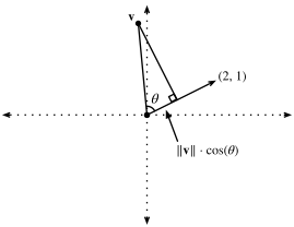
Follow the perpendicular from the tip of v to the line: its foot gives the closest point on that line. The remaining segment is the residual. This is the geometry behind least squares; this drawing uses direction (2, 1), while the constant-fit example above uses (1, 1).

Zhang et al., Dive into Deep Learning, Figure 22.1.5. · CC BY-SA 4.0

What factorizations answer

For a square matrix, $Av=\lambda v$ with $v\ne0$ identifies a vector scaled by the map (possibly to zero). Not every real matrix has real eigenvalues or enough eigenvectors to form a basis. In contrast, every real $m\times n$ matrix has a singular value decomposition $A=U\Sigma V^T$, with orthogonal $U,V$ and nonnegative singular values in rectangular $\Sigma$. The number of nonzero singular values is the rank. Keeping the largest singular values gives a best low-rank approximation in the Frobenius norm; singular values very small relative to the largest warn that solving may amplify perturbations. This connects linear algebra to numerical analysis.

My reading · Opened notes are remembered in this browser.