Machine Learning General Concepts

Model, Parameters, and Hyperparameters

A model $f_{\theta}$ maps an input $x$ to a prediction using learned parameters $\theta$. A hypothesis class is the set of functions reachable by the chosen representation. Hyperparameters—such as regularization strength, tree depth, or architecture width—control the learning procedure or hypothesis class rather than being fitted in the same inner optimization.

Loss and Empirical Risk

A per-example loss measures disagreement between a prediction and target:

$$\ell\!\left(f_{\theta}(x_i),y_i\right).$$

Training commonly minimizes empirical risk plus a regularizer:

$$J(\theta) = \frac{1}{n}\sum_{i=1}^{n} \ell\!\left(f_{\theta}(x_i),y_i\right) + \lambda\,\Omega(\theta).$$

Here $n$ is the number of training examples, and $(x_i,y_i)$ is the input–target pair for example $i$. The average loss is the empirical risk: error measured on those observed examples. The regularizer $\Omega(\theta)$ penalizes properties of the parameters, such as large coefficients, and $\lambda$ controls its weight relative to the average loss. $J$ is often called the cost or objective. When comparing objectives, check the data split, averaging convention, and penalty rather than relying on the name.

Common losses encode different assumptions:

Task	Example loss	Important boundary
regression	squared error	strongly weights large residuals
binary probabilistic classification	binary cross-entropy / logistic loss	expects a probability model or logit interpretation
mutually exclusive multiclass	softmax cross-entropy	not the same as multilabel classification
margin classification	hinge loss	optimizes a margin, not calibrated probability by itself

Loss versus a Reported Metric

Loss drives fitting; a metric judges a stated use on a stated split. They may be the same function, but need not be. For targets $(0,0,1,1)$, consider predicted positive-class probabilities:

Model	Probabilities	Accuracy at threshold 0.5	Mean log loss
A	$(0.1,0.4,0.6,0.9)$	100%	about 0.308
B	$(0.01,0.49,0.51,0.99)$	100%	about 0.342

Here log loss is $-\frac14\sum_i[y_i\log p_i+(1-y_i)\log(1-p_i)]$, with natural logarithms. Accuracy hides B's weaker probabilities on the middle cases. Conversely, a lower log loss does not guarantee lower operational cost at a fixed review capacity. The scikit-learn metric guide distinguishes these evaluation targets.

With no useful features, a training-mean constant minimizes squared error, a training median minimizes absolute error, and a majority-class rule is an accuracy baseline. Estimate these constants on training data, then compare every model on the same held-out cases.

Likelihood

For a probabilistic model $p_{\theta}(y\mid x)$, maximum likelihood chooses parameters that make the observations probable:

$$\hat{\theta}_{\mathrm{ML}} = \arg\max_{\theta} \sum_i \log p_{\theta}(y_i\mid x_i).$$

Minimizing negative log-likelihood is therefore equivalent to maximizing likelihood. The chosen likelihood determines the corresponding loss; it should follow the observation model rather than be selected only because a library exposes it.

This sum assumes observations are conditionally independent given their inputs and parameters. Dependent sequences require a joint or sequential likelihood instead. Independent Gaussian errors with a common fixed variance give squared-error loss (up to a positive factor and a constant); Bernoulli observations give binary cross-entropy.

Prediction-time inference means evaluating a fitted model on new inputs without updating its parameters. Statistical inference means drawing conclusions about unknown quantities with uncertainty. Neither is the same as optimization, which is the numerical search for parameters.

Optimization

Gradient descent updates parameters in the direction opposite the objective gradient. The learning rate $\eta>0$ sets the step size; too large a step can increase the objective or cause divergence:

$$\theta \leftarrow \theta-\eta\nabla J(\theta).$$

• Batch gradient descent uses the full training set per update.
• Stochastic gradient descent uses one sampled example.
• Minibatch methods estimate the gradient from a small batch and are the usual computational compromise.

Newton's method uses local curvature:

$$\theta \leftarrow \theta-\left[\nabla^2J(\theta)\right]^{-1}\nabla J(\theta).$$

It can converge quickly near a well-behaved optimum, but forming or solving with the Hessian can be expensive or unstable. An optimizer finding a low training objective does not prove good generalization.

Generalization Boundary

Training error, validation error, and test error answer different questions. Hyperparameter choices consume validation information; the test set should remain outside that loop. Evaluation must also consider distribution shift, leakage, subgroup behavior, uncertainty, and the cost of different errors.

Open full-size image

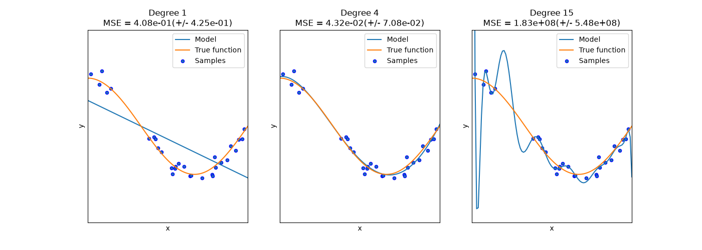
Compare the blue fitted curve with the orange data-generating function. Degree 1 misses the curvature; degree 4 follows it; degree 15 bends sharply around the noisy observations. The degree is a hyperparameter. The displayed MSE is measured by cross-validation, not training error: fitting the observed points more closely need not improve predictions on unseen points.

scikit-learn developers, Underfitting vs. Overfitting. · BSD 3-Clause

For a first model, continue with linear regression. For the mechanics shared by neural-network training, read gradients and optimizers; for a different hypothesis class, compare trees and boosting. Berkeley CS 189 provides the external course sequence.

My reading · Opened notes are remembered in this browser.