Gradient Descent in One Variable

Gradient descent iteratively seeks a minimum. To maximize $f$, minimize $-f$ instead. This approach is foundational in optimization problems where exact solutions are challenging to derive analytically, especially due to complexities in higher dimensions.

Concept of Gradient Descent

• Initially demonstrated in a single-variable context to ease into the more complex multi-variable gradient descent.
• Employs an iterative process to approximate the minimum of a function by systematically updating the point of interest based on the function's derivative.

Mathematical Formulation

Given a function $f(x) = e^x - \log(x)$, finding its minimum involves:

1. Derivative Calculation: The first step is to compute the derivative $f'(x) = e^x - \frac{1}{x}$.
2. Iterative Update: Starting from an initial point $x_0$, the next point $x_{1}$ is determined by $x_{1} = x_{0} - \alpha \cdot f'(x_{0})$, where $\alpha$ is the learning rate.

This method leverages the derivative to guide the direction of steps taken towards the minimum. The sign of the derivative indicates whether to move left or right (in the case of a single variable).

Challenges and Solutions

Analytical Difficulty

• Directly solving $e^x = \frac{1}{x}$ for $x$ is analytically challenging, exemplifying situations where gradient descent offers a practical solution.

Learning Rate ($\alpha$)

• The learning rate $\alpha$ is critical in ensuring the iterative steps are appropriately sized to prevent overshooting or excessively slow convergence.
• Adaptive Learning Rates: Research into adaptive learning rates seeks to dynamically adjust $\alpha$ based on the optimization progress, though a universally optimal strategy is yet to be established.

Open full-size image

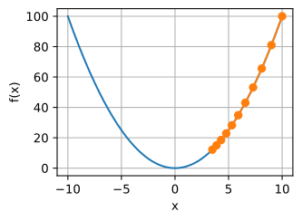
Here f(x) = x², the start is x = 10 and the learning rate is 0.05. Orange points show ten updates: they move toward zero but only reach about 3.49. This separate quadratic example illustrates small steps; the function earlier on this page is eˣ − log(x).

Zhang et al., Dive into Deep Learning, Gradient Descent — Learning Rate. · CC BY-SA 4.0

Open full-size image

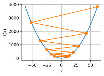
With the same function and start but a learning rate of 1.1, the iterates cross zero and grow in magnitude. The update is x ← −1.2x, so the distance increases by 20% each time. Compare axis scales: this plot covers much larger values than the one above.

Zhang et al., Dive into Deep Learning, Gradient Descent — Learning Rate. · CC BY-SA 4.0

Local Minima

• Gradient descent may converge to local minima, potentially missing the global minimum.
• Multiple Initial Points: Employing multiple starting points and running gradient descent iterations from each can enhance the likelihood of approaching the global minimum.

Practical Implementation

1. Initialization: Choose a starting point and learning rate.
2. Update Rule: Apply the update $x_{k} = x_{k-1} - \alpha \cdot f'(x_{k-1})$ iteratively.
3. Convergence Criterion: Check the derivative magnitude, objective decrease, domain validity, and an iteration limit. Small changes in $x$ alone do not establish optimality.

Example

• For $f(x) = e^x - \log(x)$, starting from an initial guess, iterations proceed by computing the derivative at the current point and updating the point according to the learning rate and the computed gradient.
• This process does not require solving for when the derivative equals zero but rather iteratively adjusts based on the gradient's direction and magnitude.

A domain-safe calculation

Here $\log$ is the natural logarithm and the domain is $x>0$. The curvature $f''(x)=e^x+1/x^2>0$ makes $f$ strictly convex. Moreover, $f$ tends to infinity as $x\to0^+$ or $x\to\infty$, so it has a unique global minimizer. Solving $xe^x=1$ gives $x_*\approx0.567143$ (also denoted $W(1)$); the warning about competing local minima does not apply to this example.

From $x_0=1$ with $\alpha=0.1$, $g_0=e-1$ and $x_1\approx0.828172$, lowering $f$ from $2.718282$ to $2.477665$. But from $x_0=2$ with $\alpha=1$, the next point is negative, so evaluating its logarithm is invalid. Reject infeasible steps before evaluating the objective. The following backtracking search halves the step until it satisfies the Armijo decrease condition; the iteration and trial caps report failure rather than claiming convergence.

from math import exp, log, isfinite

def f(x):
    return exp(x) - log(x)

x = 1.0
for iteration in range(10000):
    g = exp(x) - 1 / x
    if abs(g) <= 1e-7:
        break
    alpha = 1.0
    for trial in range(60):
        candidate = x - alpha * g
        if candidate > 0 and isfinite(candidate):
            try:
                value = f(candidate)
            except OverflowError:
                value = float("inf")
            if isfinite(value) and value <= f(x) - 1e-4 * alpha * g * g:
                break
        alpha *= 0.5
    else:
        raise RuntimeError("line search failed")
    x = candidate
else:
    raise RuntimeError("iteration limit reached")
print(round(x, 6), round(f(x), 6))

The output is 0.567143 2.330366. The derivative tolerance certifies approximate stationarity here; strict convexity identifies the only stationary point as the global minimum. For a nonconvex objective, a small derivative could instead signal a saddle or maximum.

For a step-size benchmark, $f(x)=x^2$ gives $x_{k+1}=(1-2\alpha)x_k$. For nonzero initial $x$, convergence requires $0<\alpha<1$; at $\alpha=1$ it oscillates, and above $1$ it diverges. Conversely, an extremely small $\alpha$ can make the iterate change tiny while $|f'(x)|$ remains large. If $|f'(u)-f'(v)|\le L|u-v|$ on an interval containing the step (an $L$-Lipschitz gradient), the descent bound is $f(x-\alpha g)\le f(x)-\alpha(1-L\alpha/2)g^2$, so $0<\alpha<2/L$ ensures descent when $g\ne0$. For the logarithmic example there is no single finite global $L$ on $(0,\infty)$; backtracking avoids assuming one.

My reading · Opened notes are remembered in this browser.