Decision Trees, Random Forests, and Gradient Boosting

A linear model adds feature contributions using fixed coefficients. A decision tree instead partitions the input space: follow threshold tests until reaching a leaf, then use the leaf’s prediction. This makes conditional rules easy to express—for example, request length matters only when the request also contains an attachment.

The scikit-learn tree guide describes greedy partitioning and the tendency of unconstrained trees to overfit. The word greedy matters: a split is chosen for its immediate improvement, not by exhaustively searching every possible future tree.

Open full-size image

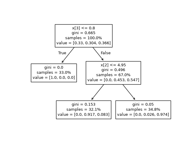
Start at the top: a true threshold test sends the sample left, a false one right. Here samples is the percentage of all training samples reaching that node, while value gives class proportions within it. A leaf predicts the class with the largest proportion. The pure left leaf has Gini = 0. This Iris example has three classes; the hand calculation below uses two.

scikit-learn developers, Understanding the decision tree structure. · BSD 3-Clause

Calculate a split

Consider four invented cases with a numeric feature $x=(1,2,3,4)$ and labels $y=(0,0,1,1)$. The parent has equal class proportions. Its Gini impurity is

$$I=1-\sum_kp_k^2=1-0.5^2-0.5^2=0.5.$$

A threshold at $2.5$ produces two pure leaves, so weighted child impurity is zero and the gain is $0.5$. A threshold at $1.5$ produces a pure one-example leaf and a three-example leaf with class proportions $(1/3,2/3)$. Its weighted impurity is $\frac34(1-1/9-4/9)=1/3$, and the gain is only $1/6$.

from collections import Counter

def gini(labels):
    n = len(labels)
    return 1 - sum((count / n) ** 2 for count in Counter(labels).values())

x, y = [1, 2, 3, 4], [0, 0, 1, 1]
for threshold in (1.5, 2.5, 3.5):
    left = [label for value, label in zip(x, y) if value <= threshold]
    right = [label for value, label in zip(x, y) if value > threshold]
    score = (len(left) * gini(left) + len(right) * gini(right)) / len(y)
    print(threshold, round(gini(y) - score, 6))

The best training split is obvious in this example. It does not establish that the threshold will transfer to new data. A tree allowed to keep splitting may isolate each noisy observation, yielding excellent training purity and poor held-out predictions. Minimum leaf size, maximum depth, and pruning restrict that behavior.

What a tree assumes about the input

Ordinary axis-aligned trees test one feature at a time. They can express interactions through successive branches, but a diagonal boundary may need many small rectangles. A linear classifier may express that same diagonal with one coefficient vector. Thus a tree is not simply a more powerful replacement for a linear model; its preferred geometry differs.

Monotonic rescaling of one numeric feature usually preserves the order of candidate splits, apart from numerical and implementation effects. Standardization is therefore less central than for distance-based clustering. However, converting categorical values to arbitrary integers introduces an order that may be meaningless. Use the estimator’s documented categorical handling or an appropriate encoding.

A regression leaf commonly predicts a mean. Outside the observed feature range, a standard regression tree routes an input to an existing leaf rather than extending a slope. That can be useful for bounded decisions but poor for extrapolating a physical trend. Do not infer “twice the input means twice the output” from its training fit.

Why a forest averages trees

Bagging fits models on resampled datasets and aggregates predictions. A random forest also randomizes feature candidates during splitting, helping make trees less correlated. The ensemble guide explains this contrast with sequential boosting.

An elementary variance calculation shows why diversity matters. Suppose $M$ prediction errors each have variance $\sigma^2$ and pairwise correlation $\rho$. The variance of their average is

$$\operatorname{Var}(\bar e)=\sigma^2\left(\rho+\frac{1-\rho}{M}\right).$$

With 100 equally noisy trees and $\rho=0.5$, the average still has $0.505\sigma^2$ variance. Adding more almost-identical trees cannot remove shared error. This calculation assumes equal variance and correlation; it explains the mechanism, not an empirical guarantee for every forest.

Boosting learns corrections

Gradient boosting adds models sequentially. At each stage, a new tree approximates a direction that reduces the chosen loss. For squared error that direction is the residual. Other objectives use their corresponding negative gradients rather than raw prediction errors.

Take targets $(1,1,3,3)$ and start with the constant mean $F_0=2$. Residuals are $(-1,-1,1,1)$. A stump separating the first two cases from the last two can fit them exactly. With shrinkage $\eta=0.5$,

$$F_1(x)=F_0(x)+0.5h_1(x),$$

so predictions become $(1.5,1.5,2.5,2.5)$. Mean squared error falls from $1$ to $0.25$. Another half correction gives $(1.25,1.25,2.75,2.75)$ and MSE $0.0625$. These are hand-computed training results on a constructed example. Noise changes the value of continuing to fit residuals, which is why validation-based early stopping matters.

Tree depth controls the interactions each correction can express; number of stages and learning rate jointly control how far the ensemble moves. A smaller rate with the same number of stages may simply underfit. Evaluate them together rather than treating one setting as universally conservative.

A fair tabular comparison

For structured data, compare a simple baseline, a regularized linear model, and one tree ensemble using the same split and features available at prediction time. Prevent repeated entities and future observations from leaking between partitions. Fit encodings only on training folds.

For imbalanced decisions, accuracy may reward ignoring the rare class. Compare class-specific errors and probability quality; changing the decision threshold may be more useful than adding trees. Leaf class frequencies and ensemble averages are not automatically calibrated for a shifted deployment population. See probability calibration.

A feature’s importance score also does not establish causation. Correlated features can substitute for each other; identifier-like features can exploit dataset artifacts. Perturbation checks and errors by subgroup help reveal what the fitted rule depends on. For the statistical meaning of coefficients and regularization in the linear baseline, continue with ordinary least squares.

My reading · Opened notes are remembered in this browser.