Clustering and Dimensionality Reduction

Clustering asks which observations should be grouped under a chosen similarity measure. Dimensionality reduction asks how to represent observations with fewer coordinates. They can be combined, but neither supplies a semantic category merely by producing a visually neat result.

For example, grouping document embeddings might help inspect recurring topics. Compressing those embeddings to two coordinates might help plot them. The plotted groups could reflect language, length, source website, or the topic you care about. Understanding them requires inspecting the original documents.

Distance is part of the model

Suppose each observation has a duration in seconds and a rating from one to five. In raw Euclidean distance, a difference of 100 seconds can dominate a difference of two rating points. Standardizing each feature changes that geometry; it does not reveal a uniquely correct distance. Choose scaling according to the comparison the task needs and estimate its statistics on the fitting data.

For unit-normalized vectors $u,v$,

$$\|u-v\|_2^2=2-2u^\top v.$$

Thus Euclidean nearest-neighbor ordering matches cosine-similarity ordering for these normalized vectors. Without normalization that equivalence does not hold. Nor does it make every clustering algorithm interchangeable: the location and normalization of cluster centers also matter. The embedding comparison explains what the vector model contributes before clustering begins.

K-means alternates assignment and averaging

K-means minimizes within-cluster squared distance to $K$ centers. A usual iteration assigns each observation to its nearest center, then replaces each center with the mean of assigned observations. The process can converge to a local solution, so initialization matters.

For invented one-dimensional data $(0,1,9,10)$, initialize centers at 0 and 10. The assignments are $(0,1)$ and $(9,10)$, whose means are $0.5$ and $9.5$. The within-cluster squared-error sum is then $4\times0.5^2=1$. With only one cluster, the center is 5 and the sum is $25+16+16+25=82$. More clusters can reduce this objective even when the extra groups have no useful interpretation.

points = [0.0, 1.0, 9.0, 10.0]
centers = [0.0, 10.0]
for _ in range(5):
    groups = [[] for _ in centers]
    for value in points:
        nearest = min(range(len(centers)), key=lambda j: (value - centers[j]) ** 2)
        groups[nearest].append(value)
    centers = [sum(group) / len(group) if group else old
               for group, old in zip(groups, centers)]
assert centers == [0.5, 9.5]
print(centers)

This example keeps an old center if its group is empty; production implementations have explicit empty-cluster policies. It illustrates the algorithm rather than serving as a general clustering package.

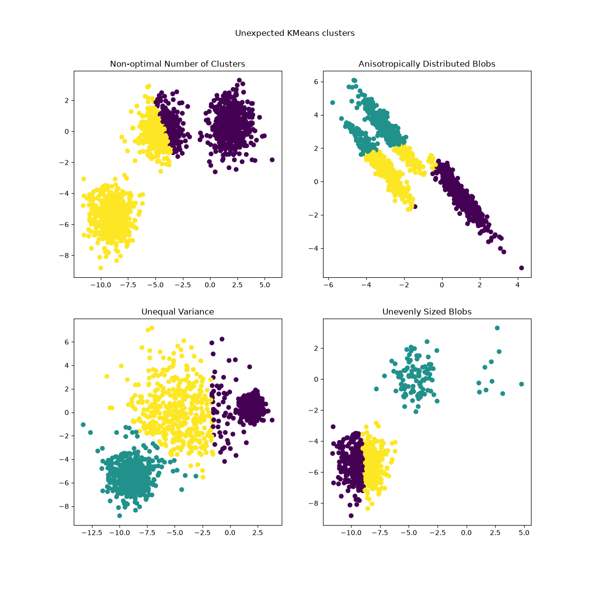
K-means prefers compact groups around means and requires $K$ in advance. Unequal densities, elongated shapes, outliers, and an unhelpful distance metric can all produce misleading partitions. Density-based methods such as DBSCAN instead connect dense neighborhoods and can leave points as noise, but their neighborhood scale remains a substantive choice. Hierarchical clustering yields nested merges; the linkage rule determines what counts as close between groups.

Open full-size image

Colors show the assignments returned by K-means. Compare elongated groups, unequal spreads and unequal group sizes: minimizing distance to a center can cut across the grouping you expected. These panels illustrate different failure cases; they are not four views of the same dataset.

scikit-learn developers, Demonstration of k-means assumptions. · BSD 3-Clause

PCA preserves variation, not labels

Principal component analysis (PCA) finds orthogonal directions of variation in centered data. Keeping the leading directions gives a lower-dimensional linear representation and a reconstruction of the original coordinates. It does not consult class labels.

Take the points $(1,1),(2,2),(3,3)$. Their mean is $(2,2)$; after centering they are $(-1,-1),(0,0),(1,1)$. The leading unit direction is

$$v_1=\frac{1}{\sqrt2}(1,1).$$

Projecting onto it gives $(-\sqrt2,0,\sqrt2)$. Multiplying each scalar by $v_1$ and adding the mean reconstructs every original point exactly. Variation along the perpendicular direction $(1,-1)/\sqrt2$ is zero. One coordinate is sufficient because this constructed dataset lies on a line.

Now imagine a second dataset where document length causes huge variation, but a small feature distinguishes duplicate from original text. PCA can discard that small direction even if it is decisive for the classification task. High explained variance therefore does not establish preserved task quality. Evaluate a downstream model with and without reduction on the same held-out examples.

A two-dimensional plot is a view

Nonlinear embeddings such as t-SNE prioritize particular neighborhood relationships rather than preserving every global distance. A large visual gap or a small-looking cluster can depend on hyperparameters and initialization. Do not estimate a category’s real-world prevalence from the area it occupies on a plot.

For an inspection workflow, retain the original vectors and document identifiers, fit the visualization, then sample points from apparent groups and boundaries. Check whether grouping survives plausible changes in preprocessing or sampling. If colors represent known labels, keep clear that the labels were added for inspection rather than discovered by the algorithm.

Evaluating something without class labels

An internal score such as silhouette compares within-group and between-group distances under the chosen metric. It can favor a geometric structure that is irrelevant to the use case. If a document collection is being organized for browsing, also measure whether people can find desired material and whether representative documents explain each group.

When reference labels exist, external agreement metrics can compare partitions while ignoring arbitrary cluster-number permutations. Even then, disagreement may reflect a different valid grouping: a dataset labeled by topic may be clustered by language. Decide which distinction is useful before calling the result wrong or right.

For downstream prediction, fit scaling and dimensionality reduction on training data only, then transform validation and test data. Fitting PCA before the split allows the representation to learn the evaluation distribution. For a descriptive plot of the full collection, using the full collection can be intentional; do not then present that plot as an independent predictive test.

Once reliable labels emerge from inspection, a supervised classifier or tree model can learn the intended distinction directly. Clustering remains useful for exploration, but assigning a number to a group does not turn it into a validated decision label.

Use the interactive examples in How to Use t-SNE Effectively to vary perplexity and optimization steps on the same data. Compare cluster sizes and distances across settings before interpreting a plot; the article shows why a visually separated island need not represent a stable, well-separated group in the original space.

My reading · Opened notes are remembered in this browser.