Probability Calibration, Decision Thresholds, and Abstention
Ten consecutive outputs of 0.99 do not establish reliability. First identify the event being predicted, then compare predictions with observed frequencies across similar cases. Classification accuracy, calibration, and whether to execute an action are related but different questions.
A probability needs a defined event
Suppose a fictional classifier predicts that a support message needs human handling, with p = 0.8. Good calibration means that among comparable messages assigned probabilities near 0.8, approximately 80% actually need human handling. It neither guarantees this particular prediction nor means the model understood 80% of the content. The scikit-learn calibration guide explains this frequency interpretation.
In multiclass systems, confidence may mean the largest class probability. Elsewhere it may denote entropy, a margin, or a separate prediction head. Read the definition first: concentrating all probability on a wrong choice can still produce high confidence. Choice probabilities in Jev and Laya must be interpreted within their interfaces and target tasks.
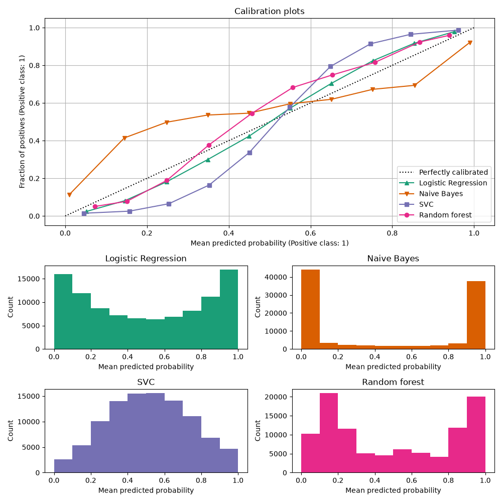 Open full-size image
In the upper plot, perfect calibration lies on the diagonal. At a given predicted probability, a curve below it indicates fewer positives than predicted. The lower panels show how many predictions occupy each range. These are results on one example dataset, not a universal ranking of classifiers.
Accuracy and confidence can disagree
Imagine 100 independently labeled examples. The model assigns 0.9 to every selected class but is correct only 70 times. Accuracy is 70%; average confidence is 90%. Changing every confidence to 0.7 can leave all selected classes unchanged while improving this group's frequency agreement.
Conversely, always predicting the dataset's positive rate may be calibrated overall while failing to distinguish individual cases. Examine discrimination as well as calibration. Guo et al. studied overconfidence in neural networks and temperature scaling of their outputs.
A positive temperature T replaces softmax(z) with softmax(z / T). One shared positive temperature preserves class ordering but changes concentration. Fit it on calibration data rather than lowering confidence by intuition. It cannot repair missing candidates, incorrect labels, or an unlearned task.
Assign separate roles to data
Training data learns the model; calibration data fits the probability mapping; validation data can select thresholds and abstention rules; a final test set evaluates the fixed system. Cross-validation can help with scarce data, but labels evaluating a prediction must not have participated in fitting or selecting that prediction.
Near-duplicate messages from one customer, or passages from one document, should not be scattered randomly across sets and treated as independent examples. A future deployment may require a temporal split. If the positive rate changes after deployment, old probabilities and thresholds can fail even when ranking remains good.
A reliability diagram compares mean probability with observed frequency in bins and should show bin counts. ECE summarizes bin gaps but depends on binning and sample size. Brier score and log loss evaluate overall probabilistic predictions; neither alone proves better calibration. This fictional binary example computes Brier score:
probabilities = [0.9, 0.8, 0.7, 0.1]
labels = [1, 1, 0, 0]
brier = sum((p - y) ** 2 for p, y in zip(probabilities, labels)) / len(labels)
print(round(brier, 4))  # 0.1375
The confidently wrong third example contributes 0.49, most of the total squared error. Four examples explain the calculation; they cannot estimate a deployed system's calibration.
Derive thresholds from consequences
Suppose an unnecessary action costs 9, a missed necessary action costs 1, and correct decisions cost 0. With a reliable probability p that the action is needed, acting costs 9(1-p) in expectation, while not acting costs p. Act when the former is smaller: p > 0.9.
This is a simplified binary cost model. Add delay, human review, and alternative actions when relevant. Probabilities estimate outcomes, costs express consequences, and permissions determine allowed actions. None substitutes for another.
Report coverage alongside abstention quality
A system can defer uncertain requests to a person or retrieve more evidence. If it reports 99% accuracy on automatically accepted requests, it must also report how many requests it accepts. Covering the easiest 1% differs substantially from covering 90%.
Raise the threshold gradually and examine the relationship between coverage and error among accepted requests, broken down by language, length, and task type. Confident out-of-distribution errors can still pass a threshold; abstention does not replace input-scope checks. When deployment data shifts, collect representative labels and reevaluate the whole decision policy instead of merely increasing the threshold.