Statistics and Probability

Probability starts with a model and reasons about possible observations. Statistics starts with observations and reasons back toward a process, parameter, or decision.

Durable Sequence

1. events, counting, conditional probability, and independence;
2. random variables, distributions, expectation, variance, and covariance;
3. laws of large numbers and the central limit theorem;
4. sampling, estimators, uncertainty, and confidence intervals;
5. hypothesis tests, effect sizes, and multiple comparisons;
6. experiment design and sample-size planning.

This reference covers elementary probability models and inference from repeated sampling. It does not develop regression, causal inference, or a full testing procedure. Harvard Statistics 110 supplies the longer probability course.

Events, conditioning, and independence

A probability model specifies possible outcomes, events (sets of outcomes), and probabilities. Probabilities are nonnegative, the whole outcome space has probability 1, and probabilities add for disjoint events. “Favorable cases divided by total cases” applies only to equally likely elementary outcomes.

Conditional probability is $P(A\mid B)=P(A\cap B)/P(B)$ when $P(B)>0$. Events are independent when $P(A\cap B)=P(A)P(B)$. Disjoint positive-probability events are not independent: observing one rules out the other. Bayesian updating uses conditioning to move from prior probabilities and likelihoods to a posterior; $P(A\mid B)$ and $P(B\mid A)$ generally differ.

Random variables and distributions

A random variable assigns a number to each outcome. Its distribution describes those numbers' probabilities. For a discrete variable, the mass function $p(x)$ sums to 1. For a continuous variable with density $f$, probabilities are integrals: $P(a\le X\le b)=\int_a^b f(x)\,dx$. A density value is not a point probability; $P(X=x)=0$, and a density can exceed 1.

Model	Meaning and assumptions	Mean and variance
Bernoulli$(p)$	One indicator, 1 for success and 0 otherwise, $0\le p\le1$	$p$; $p(1-p)$
Binomial$(n,p)$	Number of successes in $n$ independent Bernoulli trials with the same $p$	$np$; $np(1-p)$
Normal$(\mu,\sigma^2)$	Continuous bell-shaped model, $\sigma>0$	$\mu$; $\sigma^2$
Exponential$(\lambda)$	Nonnegative waiting time with constant rate $\lambda>0$	$1/\lambda$; $1/\lambda^2$

A model is an assumption to assess, not a label justified by a histogram alone. Sampling without replacement from a small finite population does not produce independent Bernoulli trials.

Expectation and variation

Expectation is a probability-weighted average: $E[X]=\sum_x xp(x)$ in the discrete case, or $\int x f(x)\,dx$ for a density, provided $E[|X|]$ is finite. Variance is $\operatorname{Var}(X)=E[(X-E[X])^2]$ when the second moment is finite. Standard deviation is its square root and has the same units as $X$.

For a fair die, $E[X]=3.5$ and $E[X^2]=91/6$, so $\operatorname{Var}(X)=91/6-3.5^2=35/12$. The expectation need not itself be a possible outcome. Linearity gives $E[X+Y]=E[X]+E[Y]$ without independence, whereas

$$\operatorname{Var}(X+Y)=\operatorname{Var}(X)+\operatorname{Var}(Y)+2\operatorname{Cov}(X,Y).$$

Here covariance is $E[(X-E[X])(Y-E[Y])]$. Independence implies zero covariance when second moments exist, but zero covariance does not generally imply independence.

A two-asset example in Returns, Diversification, and Portfolio Risk applies covariance to portfolio volatility.

From a sample to an estimate

For independent, identically distributed observations with mean $\mu$ and finite variance $\sigma^2$, the sample mean is unbiased: $E[\bar X]=\mu$. Its variance is $\sigma^2/n$ and its standard error is $\sigma/\sqrt n$. Standard deviation describes individual observations; standard error describes the estimator across repeated samples.

For example, 100 independent Bernoulli trials with $p=0.5$ have a sample-proportion standard error of $0.05$. About two standard errors gives a rough 95% normal-approximation interval half-width of $0.10$. A 95% confidence procedure covers the fixed true parameter in 95% of repetitions under its assumptions; it does not assign a 95% posterior probability to that parameter in one observed interval.

The law of large numbers explains convergence of averages to the expectation; the central limit theorem describes the limiting shape of standardized fluctuations. Neither removes sampling bias. More responses from a systematically excluded or self-selected population can make a biased estimate more precise. Specify the target population and sampling mechanism before using sample-size formulas; random assignment of treatment addresses a different question from random selection into a sample.

Open full-size image

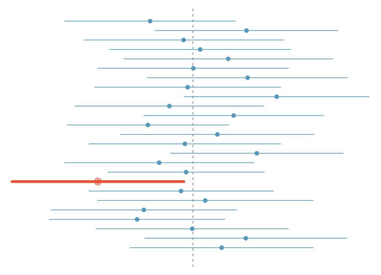
Each horizontal segment comes from a different sample; the vertical dashed line is the fixed population mean. The interval drawn with a hollow point misses it. Coverage describes repeated sampling: this illustration happens to show 24 successes out of 25, not a requirement that every batch contain exactly 95% successful intervals.

OpenIntro Statistics, 2nd ed., Chapter 4 slides, slide 15 (figure crop). · CC BY-SA 3.0

In Seeing Theory’s confidence-interval experiment, select a population distribution, sample size, and confidence level, then generate repeated intervals. Compare their widths and whether they cover the fixed population mean; changing the confidence level changes the procedure, not the parameter.

Confidence intervals from observed data

Suppose measurements are independent draws from a normal population with unknown mean and variance. The NIST interval for the mean uses the observed sample mean $\bar x$ and sample standard deviation $s$, calculated with denominator $n-1$:

$$\bar x\pm t_{0.975,n-1}\frac{s}{\sqrt n}.$$

Here $t_{0.975,n-1}$ is the 97.5th percentile of Student's t distribution with $n-1$ degrees of freedom. For the illustrative observations [8, 9, 10, 11, 12], $\bar x=10$, $s^2=10/4=2.5$, and $s/\sqrt5\approx0.7071$. Using $t_{0.975,4}\approx2.7764$ gives a 95% interval of approximately $[8.037,11.963]$. Normality and independence justify exact coverage here; five observations cannot establish these assumptions. This is an interval for the population mean, not a range containing 95% of individual future observations.

Bootstrap and paired model comparisons

When a useful analytic interval is unavailable, a nonparametric bootstrap approximates repeated sampling by drawing, with replacement, $n$ observations from the observed sample and recomputing the statistic many times. A percentile interval uses the 2.5th and 97.5th percentiles of those statistics. It is an approximation, not an exact guarantee; skew, bias, sparse outcomes, or degenerate samples can make it unreliable. SciPy's bootstrap documentation explains percentile, basic, and bias-corrected and accelerated (BCa) intervals.

To compare two fixed models on the same independent test cases, compute a per-case loss difference $d_i=\ell_A(i)-\ell_B(i)$. Positive mean difference favors B when lower loss is better. Resample case indices and keep each pair together; separately resampling A and B discards their paired dependence. A percentile interval for the mean difference that includes zero does not establish equivalence. A useful comparison also asks whether the magnitude matters for the intended decision.

The resampling unit must follow the sampling design. Repeated observations from one person call for cluster-aware inference; dependent time observations may need suitable blocks and assumptions about temporal stability. Resampling fixed predictions measures test-sample uncertainty, not variation from refitting the models or future distribution shift. More bootstrap repetitions reduce simulation noise, not bias in the original sample. Apply these distinctions when evaluating models under distribution shift.

My reading · Opened notes are remembered in this browser.