Linear and Quadratic Discriminant Analysis

Linear discriminant analysis (LDA) and quadratic discriminant analysis (QDA) model each class with a Gaussian distribution and combine the class-conditional density with a class prior $\pi_k$.

For class $k$,

$$p(x\mid y=k) = \mathcal{N}(x;\mu_k,\Sigma_k).$$

Ignoring terms shared by all classes, the discriminant score is

$$\delta_k(x) = -\frac{1}{2}\log|\Sigma_k| -\frac{1}{2}(x-\mu_k)^{\top}\Sigma_k^{-1}(x-\mu_k) +\log\pi_k.$$

The predicted class has the largest score.

From Training Data to a Decision

Bayes' rule gives the posterior:

$$p(y=k\mid x)=\frac{\pi_k p(x\mid y=k)}{\sum_j\pi_j p(x\mid y=j)} =\frac{e^{\delta_k(x)}}{\sum_j e^{\delta_j(x)}}.$$

Estimate each mean from its training class, and estimate priors as $n_k/n$ unless justified target-population priors are supplied. One explicit maximum-likelihood convention estimates $\Sigma_k$ by dividing the within-class sum of outer products by $n_k$; LDA pools those sums across classes and divides by $n$. Unbiased covariance conventions instead use $n_k-1$ or $n-K$; state the convention, since implementations need not match this calculation.

For a one-dimensional example, class 0 has training values $(-1,1)$ and class 1 has $(1,3)$. The fitted means are 0 and 2, the shared ML variance is 1, and both priors are $1/2$. Hence

$$\delta_1(x)-\delta_0(x)=2x-2.$$

The boundary is $x=1$; at $x=1.5$ the posterior for class 1 is $1/(1+e^{-1})\approx0.731$. With the same means and variance but priors $\pi_1=0.1$, $\pi_0=0.9$, the boundary moves to $1+\frac12\log9\approx2.099$. A prior is not merely a label attached after fitting.

Choosing the largest posterior minimizes expected zero-one loss under the fitted model. Unequal error costs require minimizing posterior expected cost instead. Neither a Gaussian fit nor this decision rule guarantees that the model matches the deployment distribution.

LDA versus QDA

Model	Covariance assumption	Boundary	Main trade-off
LDA	one shared $\Sigma$	linear	fewer covariance parameters, stronger assumption
QDA	one $\Sigma_k$ per class	quadratic	more flexible, much more data needed for stable estimation

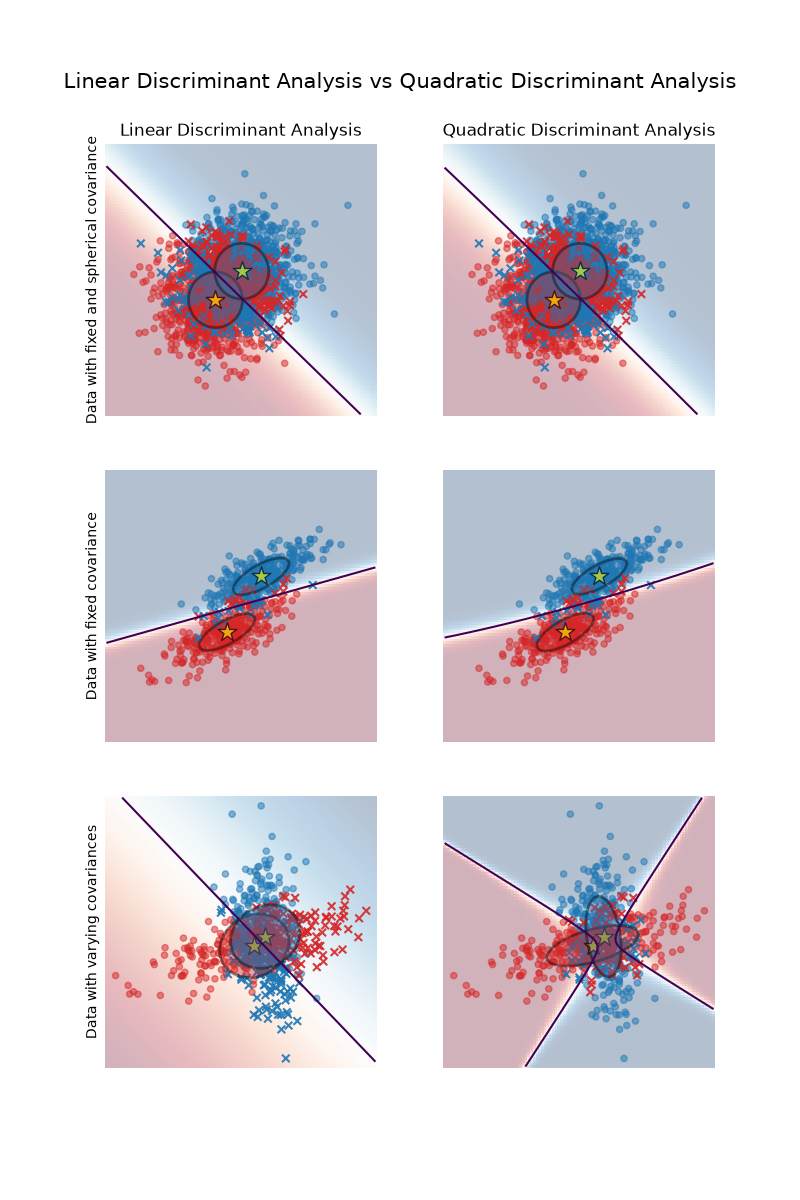
With a shared covariance, the quadratic terms in $x$ cancel between class scores, producing a linear boundary. Class-specific covariances retain those terms and produce a quadratic boundary. Class-specific diagonal covariance corresponds to a Gaussian naive Bayes-style conditional independence assumption.

Open full-size image

Compare columns within each row, then move downward as the covariance structure changes. Ellipses show estimated class spread. In the bottom row, LDA retains a straight boundary while QDA bends around classes with different covariances. Greater flexibility alone does not guarantee better predictions on new data.

scikit-learn developers, Linear and Quadratic Discriminant Analysis with covariance ellipsoid. · BSD 3-Clause

Covariance Is the Hard Part

• High-dimensional or small-sample settings can make empirical covariance matrices noisy or singular.
• Shrinkage trades some bias for more stable covariance estimates and must be selected or estimated deliberately.
• Unregularized full-covariance LDA/QDA is invariant to a common invertible affine feature transformation in exact arithmetic. Scaling still affects numerical conditioning and some regularization schemes; class imbalance affects estimated priors.
• Closed-form parameter estimates do not mean the modeling choices require no validation.

The displayed density assumes positive-definite covariances. With $d$ features, an empirical class covariance has rank at most $\min(d,n_k-1)$; QDA therefore needs at least $d+1$ observations per class even to make full rank possible, and that count is not a guarantee of stability. A pooled LDA covariance has rank at most $\min(d,n-K)$. Reduce redundant dimensions or use validated covariance regularization when these matrices are singular.

Supervised Projection

LDA can also project data onto directions that separate class means relative to within-class variation. This supervised dimensionality-reduction view is related to, but distinct from, using LDA as a classifier. With $K$ classes, at most $K-1$ discriminant directions carry between-class separation.

Gaussian assumptions can be useful approximations, but predicted probabilities still require calibration checks under the target distribution. Compare LDA and QDA with logistic regression and simple baselines rather than selecting by boundary shape alone.

See the scikit-learn LDA/QDA guide for current covariance estimators and implementation details.

My reading · Opened notes are remembered in this browser.