Ordinary Least Squares and Regularization

For the model, residuals, and step-by-step gradient updates, start with linear regression. Here the question is how to solve the least-squares problem directly, when its coefficients are identifiable, and which additional assumptions support uncertainty estimates.

For design matrix $X$, targets $y$, and coefficient vector $w$, ordinary least squares (OLS) solves

$$\hat{w}=\arg\min_w\|Xw-y\|_2^2.$$

The pseudoinverse gives a least-squares solution, $\hat{w}=X^{+}y$. When columns of $X$ are nearly linearly dependent, small changes in the data can produce large coefficient changes. Prediction may remain acceptable while individual coefficients become unstable.

From Residuals to a Solution

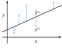
Here $X$ has $n$ rows (observations) and $p$ columns (coefficients), $y\in\mathbb{R}^n$, and $w\in\mathbb{R}^p$. Include a column of ones if an intercept is fitted. For a line $\hat y_i=b+ax_i$, the residual is $r_i=y_i-\hat y_i$: a vertical difference in target units, not the shortest distance to the line. That perpendicular distance is $|r_i|/\sqrt{1+a^2}$ in unscaled Cartesian coordinates; minimizing it would solve a different problem that also permits movement in $x$.

Open full-size image

For any point, keep x fixed and move vertically to the line: the point gives the observed y, and the line gives the predicted ŷ. Each blue segment shows the magnitude of a residual, rather than the perpendicular distance to the line. OLS chooses the line that minimizes the sum of these squared vertical differences. This D2L illustration uses its own data; the three-observation calculation below is a separate example.

Dive into Deep Learning, Figure 3.1.1 · CC BY-SA 4.0

Using $J(w)=\|Xw-y\|_2^2/(2n)$ leaves the OLS minimizers unchanged and gives

$$\nabla J(w)=\frac{1}{n}X^\top(Xw-y),\qquad \nabla^2J(w)=\frac{1}{n}X^\top X.$$

The Hessian is positive semidefinite, so a zero gradient is a global minimum. Setting it to zero gives the normal equations:

$$X^\top X\hat w=X^\top y.$$

If $\operatorname{rank}(X)=p$ (thus $n\geq p$), the solution is unique and equals $(X^\top X)^{-1}X^\top y$. Otherwise coefficients are not unique: adding any vector in the null space of $X$ leaves the fitted values unchanged. The Moore–Penrose pseudoinverse selects the minimum-Euclidean-norm coefficient vector; the training fitted values are still unique. For example, duplicate columns identify only the sum of their coefficients. Predictions outside that column relationship need not agree.

Use a QR- or SVD-based least-squares solver rather than explicitly forming an inverse; forming $X^\top X$ squares the spectral condition number for full-column-rank $X$. The scikit-learn linear-model guide describes OLS and its SVD solution.

Three Observations by Hand

Take $(x,y)=(0,1),(1,2),(2,2)$. The intercept column and $x$ column are independent. With $\bar x=1$ and $\bar y=5/3$,

$$a=\frac{\sum_i(x_i-\bar x)(y_i-\bar y)}{\sum_i(x_i-\bar x)^2} =\frac{1}{2},\qquad b=\bar y-a\bar x=\frac{7}{6}.$$

Predictions are $(7/6,10/6,13/6)$, residuals are $(-1/6,1/3,-1/6)$, and the squared-error sum is $1/6$. Both $\sum_i r_i=0$ and $\sum_i x_i r_i=0$ check the normal equations. The training-mean baseline predicts $5/3$ and has squared-error sum $2/3$. This is a training comparison, not evidence of generalization.

from math import isclose
from statistics import mean

x, y = [0, 1, 2], [1, 2, 2]
xbar, ybar = mean(x), mean(y)
sxx = sum((v - xbar) ** 2 for v in x)
if sxx == 0:
    raise ValueError("A constant x cannot identify slope and intercept separately")
a = sum((u - xbar) * (v - ybar) for u, v in zip(x, y)) / sxx
b = ybar - a * xbar
r = [v - (b + a * u) for u, v in zip(x, y)]
assert isclose(a, 0.5) and isclose(b, 7 / 6)
assert isclose(sum(v * v for v in r), 1 / 6)
assert isclose(sum(r), 0, abs_tol=1e-12)
assert isclose(sum(u * v for u, v in zip(x, r)), 0, abs_tol=1e-12)

Fitting Is Not Statistical Inference

No Gaussian assumption is needed to compute the minimizer. For statistical use, the statsmodels regression documentation makes the error covariance model explicit; choosing an uncertainty formula requires that extra model. Under a correctly specified conditional mean $y=X\beta+\varepsilon$ with $\mathbb{E}[\varepsilon\mid X]=0$ and full column rank, OLS is conditionally unbiased. If also $\operatorname{Var}(\varepsilon\mid X)=\sigma^2 I$, then

$$\operatorname{Var}(\hat w\mid X)=\sigma^2(X^\top X)^{-1}.$$

For $n>p$, residual sum of squares divided by $n-p$ estimates $\sigma^2$ under these assumptions. Conditional Gaussian errors additionally justify the usual exact finite-sample t/F inference. Heteroskedastic or correlated errors require appropriate uncertainty estimators; robust standard errors do not fix a wrong conditional mean or confounding. An interval for a mean response is not a prediction interval for a new noisy observation.

Large residuals can dominate squared error, and high-leverage observations (unusual feature values) can strongly move the fitted line. Inspect residuals against fitted values and time, and compare held-out errors with a baseline before interpreting coefficients.

Penalized Objectives

Below, $\lambda\geq0$ and $0\leq\rho\leq1$. For these penalized formulas, use training-centered $X,y$ and let $w$ contain slopes only; recover the unpenalized intercept as $\bar y-\bar x^\top w$. Scale features within training folds because coefficient penalties depend on units. Normalization is part of the definition: scikit-learn Ridge uses $\|Xw-y\|^2+\alpha\|w\|^2$, so the Ridge formula here corresponds to $\alpha=2n\lambda$. Its Lasso and Elastic Net conventions match $\alpha=\lambda$, with l1_ratio equal to $\rho$. The Ridge term at $\rho=0$ in the Elastic Net formula has half the strength of the Ridge formula below at the same $\lambda$.

Ridge

$$\hat{w}_{\text{ridge}} = \arg\min_w \frac{1}{2n}\|Xw-y\|_2^2 + \lambda\|w\|_2^2.$$

Ridge shrinks correlated or weakly identified coefficients and usually keeps all of them nonzero.

Lasso

$$\hat{w}_{\text{lasso}} = \arg\min_w \frac{1}{2n}\|Xw-y\|_2^2 + \lambda\|w\|_1.$$

The $\ell_1$ penalty can set coefficients exactly to zero. That sparsity is a property of the fitted objective, not proof that the selected variables are uniquely important or causal. With strongly correlated features, the selected member may be unstable.

Elastic Net

$$\hat{w}_{\text{EN}} = \arg\min_w \frac{1}{2n}\|Xw-y\|_2^2 + \lambda\left[ \rho\|w\|_1 + \frac{1-\rho}{2}\|w\|_2^2 \right].$$

Elastic Net combines sparsity with Ridge-style stabilization and is often useful when predictors occur in correlated groups.

Working Rules

• Fit scaling and basis transformations on training data only; apply the recorded transformation to validation and test data.
• Do not penalize the intercept unless the formulation explicitly intends it.
• Select $\lambda$ and $\rho$ using validation or cross-validation inside the training process.
• Compare predictive error, coefficient stability, and operational simplicity—not training loss alone.
• Use robust or quantile objectives when squared error does not represent the desired target or error cost.
• Separate predictive modeling from inferential claims; uncertainty estimates require explicit assumptions about the data-generating process.

Polynomial and interaction features can make the input relationship nonlinear while the fitted coefficients remain linear. The resulting model still inherits extrapolation and overfitting risks from the chosen basis.

See the scikit-learn linear-model guide for current solvers and estimator APIs.

My reading · Opened notes are remembered in this browser.