Model Evaluation Under Distribution Shift

Evaluation estimates how a system behaves under one target distribution, threshold, workflow, and error cost; it does not assign a permanent score.

For deployment distribution $Q(x,y)$ and loss $\ell$:

$$R_Q(f)=\mathbb{E}_{(x,y)\sim Q}[\ell(f(x),y)].$$

A test average estimates this risk only when test approximates $Q$, remains outside development, and uses the right labels and loss. A narrow iid interval does not include unknown future shift.

Open full-size image

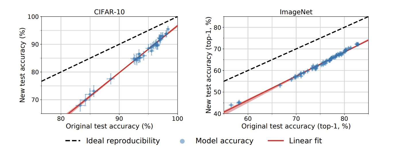
Each blue point is one model: horizontal position is its original test accuracy, vertical position its accuracy on newly collected test data. Points below the dashed diagonal lost accuracy, even though the red fitted line shows a strong relationship between the two scores. The panels cover CIFAR-10 and ImageNet; error bars are 95% Clopper–Pearson intervals. A ranking that broadly persists can coexist with a systematic drop in absolute performance.

Recht, Roelofs, Schmidt & Shankar, ImageNetV2 project: original vs. new test accuracy.

Specify the Object

system           model + preprocessing + threshold + human process
unit             one prediction object
population       people/time/place to which results extend
prediction_time  information available then
outcome_horizon  label window and maturity
action           what the prediction triggers
loss             false-positive, false-negative, delay, and abstention cost

If an action changes later data, static test evaluates the predeployment policy, not the feedback loop.

Shift Types

Type	Change	Example	Boundary
covariate	$p(x)$	device, region, season	feature drift does not prove $p(y\mid x)$ stable
label/prior	$p(y)$	disease or fraud prevalence	needs labels or assumptions
concept/conditional	$p(y\mid x)$	policy changes relationships	hard to detect from unlabeled inputs
measurement	recording process	sensor or coding change	may resemble real behavior change
selection	inclusion mechanism	only reviewed cases are labeled	test represents the selected population

They can overlap. Input drift does not guarantee performance loss, and no detected drift does not guarantee safety.

In the strict covariate-shift model, $P(x)$ changes while $P(y\mid x)$ stays fixed. Pure label shift instead changes $P(y)$ while preserving $P(x\mid y)$. These are assumptions, not conclusions from an input histogram. Reweighting source errors by $Q(x)/P(x)$ estimates target risk under covariate shift only where the source covers the target support; large weights also make estimates noisy. Reweighting cannot create evidence for feature regions never observed.

Splits Answer Different Questions

Question	Design	Main limitation
new independent same-regime cases	random holdout/CV	not time, region, or entity shift
new entities	group holdout	few groups yield wide uncertainty
future performance	rolling/forward test	covers only observed historical changes
new institution	external validation	one site is not all sites
unbiased estimate after selection	nested CV or locked test	still depends on sampling mechanism

Repeatedly viewing test, publishing only the best seed, or tuning to an external benchmark converts test into validation.

Metrics Answer Different Questions

Accuracy follows class prevalence. Precision and recall depend on threshold. Under pure prior shift with fixed class-conditional score distributions, recall stays fixed but precision changes with prevalence. ROC-AUC measures ranking, not an operating point. PR-AUC emphasizes positives but has a prevalence-dependent baseline. Log loss and Brier score assess probability quality differently. Calibration is distribution- and sample-dependent.

For regression, MAE and RMSE weight tails differently; percentage errors can fail near zero; quantile loss targets conditional quantiles. Ranking metrics describe a ranking protocol, not downstream utility. Select metrics from actions and error costs, not leaderboard convention.

Worked Example: 1% Fraud

Among 10,000 transactions, 100 are fraud. Always predicting normal gives 99% accuracy and zero recall. Suppose a threshold flags 200 transactions, 60 truly fraudulent:

precision = 60 / 200 = 30%
recall    = 60 / 100 = 60%

If nothing is flagged, precision has a zero denominator and is undefined; if a test slice contains no positives, recall is undefined. Report these cases rather than silently treating them as successful predictions.

Usefulness also depends on 200 review costs, the 40 missed cases, customer friction, delayed labels, and next month's prevalence. Select the threshold on validation, then evaluate it on a later test; selecting and reporting it on the same test is optimistic.

The false-positive rate here is $140/9900\approx1.414\%$. For prevalence $\pi$, true-positive rate $t$, and false-positive rate $f$,

$$\operatorname{precision}=\frac{\pi t}{\pi t+(1-\pi)f},\qquad \operatorname{recall}=t.$$

If prevalence rises to 5% while these conditional rates stay fixed, expected precision becomes about 69.1% and recall remains 60%. This is a prior-shift calculation, not a forecast that the conditional rates will remain stable. See the scikit-learn metric definitions.

For an operational threshold, suppose calibrated $p$ is the probability of fraud, a false alarm costs $C_{FP}>0$, a miss costs $C_{FN}>0$, and correct decisions have zero cost. Flag when $C_{FP}(1-p)<C_{FN}p$, or $p>C_{FP}/(C_{FP}+C_{FN})$. Capacity limits or nonzero review costs change this decision problem; a ROC-AUC value alone cannot choose the threshold.

Three Uncertainty Layers

1. Evaluation sample: analytic or bootstrap intervals; preserve pairing when comparing models on the same cases, and resample clusters/blocks when group or time dependence exists.
2. Training randomness: initialization, order, and nondeterministic kernels; repeat seeds.
3. Environment: future policy, behavior, sensors, and population; iid intervals usually omit it.

Report denominators, slice counts, failed runs, and which uncertainty an interval represents.

Slices, Thresholds, and Abstention

Overall metrics may hide failures by group, device, language, time, or difficulty. Predefine risk-relevant slices; many post-hoc slices create selection effects and need confirmation. High-consequence systems may abstain or route to humans, but reviewer skill, queue capacity, and selection bias become part of the system. Confidence is not automatically calibrated probability, especially under shift.

Baselines and Stress Tests

Use constants, seasonal rules, business processes, and simple models; remove suspicious features; stress time, noise, missingness, length, language, or device; test new cohorts/sites; exercise invalid input and refusal paths; and compare architectures at controlled parameter, data, and training budgets.

intended_decision: ...
target_population_and_period: ...
prediction_time_and_horizon: ...
data_version_and_split: ...
baselines: [...]
selection_metric: ...
final_metrics_and_thresholds: ...
uncertainty: sample, seed, environment
slices_and_minimum_counts: [...]
leakage_and_contamination_checks: [...]
resource_and_latency_budget: ...
known_failures_and_out_of_scope: [...]
monitoring_and_revalidation_trigger: ...

Public benchmarks support comparison but invite overfitting to fixed tasks, languages, hardware, and success metrics. Internal tests better match use but may be small and unaudited. Model Cards and the NIST AI RMF provide reporting questions; they do not certify safety or fairness.

This note concerns supervised prediction. Causal effects, A/B tests, RL policies, open-ended generation, and human–AI collaboration require different estimands and designs.

My reading · Opened notes are remembered in this browser.