Model Quantization: Precision, Size, and Speed

Quantization approximates numerical values with fewer bits. Its most direct benefit is less data to store and move. Speed and task-quality changes depend on the model, method, kernels, and hardware. Start with a memory budget, then identify what to compress rather than relying on “4-bit” in a filename.

Approximate a group of values

In symmetric uniform quantization, choose a scale s, encode a weight as q = round(w / s) within a finite integer range, and reconstruct it as s × q. Out-of-range values are clipped. Asymmetric quantization adds a zero point so the integer interval can represent a range not centered on zero.

This invented example uses a simplified symmetric 4-bit convention from -7 to 7, leaving one code unused. Real formats can use other layouts.

weights = [-1.0, -0.2, 0.3, 1.0]
scale = max(abs(w) for w in weights) / 7
quantized = [max(-7, min(7, round(w / scale))) for w in weights]
restored = [round(q * scale, 3) for q in quantized]
print(quantized)  # [-7, -1, 2, 7]
print(restored)   # [-1.0, -0.143, 0.286, 1.0]

The middle weights change. With one scale for a whole layer, a large outlier can make ordinary small weights coarsely represented. Per-channel or smaller-group scales better match local ranges but add metadata and affect kernel costs.

What is actually quantized?

The Transformers overview describes methods and backend support. Distinguish three objects:

Object	Lifetime and role	Main effect of compression
Weights	Reused across requests after loading	Storage, bandwidth, resident memory
Activations	Intermediate values in a forward pass	Compute precision, temporary memory, kernel requirements
KV cache	Grows with context and concurrent requests	Long-context capacity and reads per decoding step

Four-bit weights can coexist with 16-bit activations and cache. Computation may locally dequantize weights before using floating-point kernels. W4A16 means 4-bit weights and 16-bit activations, not that every value in the process uses four bits. File containers, quantization algorithms, and execution kernels are also distinct. A downloadable format need not run efficiently on the chosen runtime and device.

Estimate capacity without hiding overhead

An invented dense model with exactly 8 billion weights needs 8 × 10^9 × 2 = 16 GB for raw 16-bit weights and 8 × 10^9 × 0.5 = 4 GB for raw 4-bit weights. These are decimal GB, not GiB.

Files also contain scales, zero points, unquantized tensors, and metadata. Running memory adds KV cache, scratch space, runtime overhead, and concurrent requests. Four gigabytes of weights do not imply that four gigabytes of VRAM support any context length. For mixture-of-experts models, distinguish activated parameters per token from weights stored or loaded; sparse activation does not remove the total model's storage requirement.

PTQ, QAT, and calibration data

Post-training quantization approximates existing weights. Quantization-aware training incorporates quantization effects into training. Rounding illustrates the principle, while more advanced methods reduce important errors using weight and activation distributions. GPTQ uses approximate second-order information for post-training weight quantization; AWQ uses activation statistics to protect important weight channels.

Calibration data here estimates ranges or approximation errors; this differs from probability calibration. Code, long contexts, and multilingual tasks can have different activation distributions. Unrepresentative calibration text can leave a format strong on a broad benchmark but weak on the target job.

LoRA adapts a limited parameter set; distillation transfers teacher behavior to a student. Neither is numerical quantization, although they can be combined. See transfer learning, LoRA, and distillation.

Open full-size image

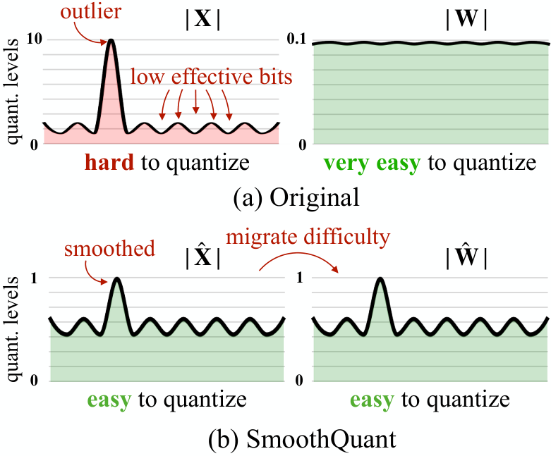
Above, an activation outlier forces most values into few quantization levels. SmoothQuant rescales activation channels and compensates in the weights, preserving the unquantized product while redistributing quantization difficulty. Compare the vertical scales as well as the shapes. This illustrates weight-and-activation quantization, distinct from the weight-only AWQ method discussed above.

Xiao et al., SmoothQuant (2023), Figure 2.

Smaller does not guarantee faster

Reduced weight traffic can help a bandwidth bottleneck. Unsupported kernels, dequantization overhead, or slow fallback operators can erase the benefit. Long-prompt prefill, token-by-token decode, and different batch sizes have different bottlenecks.

Compare formats with the original model, runtime, hardware, prompts, and output budget fixed. Record peak memory, first-token latency, generation rate, task accuracy, and failure cases. Include long text, rare terms, structured outputs, and tool arguments rather than only perplexity or casual chat. If lower precision causes repeated retries, single-inference savings can disappear at the workflow level. Inference performance explains the measurement boundaries.

My reading · Opened notes are remembered in this browser.