Improper Integrals and Numerical Integration

An improper integral uses a limit at infinity or at an unbounded singularity. A bounded function with finitely many jump discontinuities can be an ordinary Riemann integral; a discontinuity alone does not make it improper. In the definitions below, every truncated integral must exist, and convergence means that each required limit exists and is finite. See Paul Dawkins’s improper-integral treatment.

In the power-tail test assume $a>0$. Near zero the criterion is different: $\int_0^1x^{-p}\,dx$ converges exactly when $p<1$. For $p\ne1$, integrate to get $x^{1-p}/(1-p)$ and take the relevant endpoint limit; for $p=1$, use $\ln x$. Thus

$$\int_1^\infty x^{-2}\,dx=\lim_{R\to\infty}(1-1/R)=1, \qquad \int_0^1x^{-1/2}\,dx=\lim_{\varepsilon\to0^+}(2-2\sqrt\varepsilon)=2.$$

But $\int_0^1x^{-2}\,dx$ diverges. Comparison gives another useful case: $0\le1/(1+x^2)\le1/x^2$ for $x\ge1$, so its tail converges. The compared functions must be integrable on finite truncated intervals.

Do not cancel infinities across a singularity. For $1/x$ on $[-1,1]$, the left and right integrals diverge. Equal cutoffs give zero, but that is a Cauchy principal value, not convergence of the improper integral.

Improper Integrals

Improper integrals are integrals with either infinite limits or unbounded singularities. They help extend the concept of integration beyond the traditional bounds. Here's how they are defined and evaluated:

Infinite Limits

• Integral from a to infinity:

  $\int_{a}^{\infty} f(x) \, dx = \lim_{{t \to \infty}} \int_{a}^{t} f(x) \, dx$

• Integral from negative infinity to b:

  $\int_{-\infty}^{b} f(x) \, dx = \lim_{{t \to -\infty}} \int_{t}^{b} f(x) \, dx$

• Integral from negative infinity to infinity:

  $\int_{-\infty}^{\infty} f(x) \, dx = \int_{-\infty}^{c} f(x) \, dx + \int_{c}^{\infty} f(x) \, dx \quad \text{(provided both integrals are convergent)}$

Discontinuous Integrand

• Discontinuity at a:

  $\int_{a}^{b} f(x) \, dx = \lim_{{t \to a^{+}}} \int_{t}^{b} f(x) \, dx$

• Discontinuity at b:

  $\int_{a}^{b} f(x) \, dx = \lim_{{t \to b^{-}}} \int_{a}^{t} f(x) \, dx$

• Discontinuity within the interval (a < c < b):

  $\int_{a}^{b} f(x) \, dx = \int_{a}^{c} f(x) \, dx + \int_{c}^{b} f(x) \, dx \quad \text{(provided both are convergent)}$

Comparison Test for Improper Integrals

For nonnegative functions on $[a,\infty)$:

• If $0 \leq f(x) \leq g(x)$ and $\int_a^\infty g(x)\,dx$ converges, then $\int_a^\infty f(x)\,dx$ also converges.
• If $0 \leq g(x) \leq f(x)$ and $\int_a^\infty g(x)\,dx$ diverges, then $\int_a^\infty f(x)\,dx$ also diverges.

Useful Fact

For $p > 0$, the integral $\int_{a}^{\infty} \frac{1}{x^p} \, dx$ converges if $p > 1$ and diverges for $p \leq 1$.

Numerical Integration Methods

Numerical integration methods are used to approximate the value of a definite integral when it is difficult or impossible to calculate it analytically. The following are common numerical integration rules:

Midpoint Rule

The Midpoint Rule estimates the integral of a function by summing the value of the function at the midpoint of each interval, multiplied by the width of the intervals.

For $n$ subintervals, the approximation is:

$$\int_{a}^{b} f(x) dx \approx \Delta x \left[ f\left(x_1^*\right) + f\left(x_2^*\right) + \ldots + f\left(x_n^*\right) \right]$$

where $\Delta x = \frac{b - a}{n}$ and $x_i^*$ is the midpoint of the $i$-th subinterval.

Trapezoid Rule

The Trapezoid Rule calculates the integral by averaging the function values at the endpoints of each interval, effectively estimating the area under the curve using trapezoids.

The formula is:

$$\int_{a}^{b} f(x) dx \approx \frac{\Delta x}{2} \left[ f(x_0) + 2f(x_1) + 2f(x_2) + \ldots + 2f(x_{n-1}) + f(x_n) \right]$$

Simpson's Rule

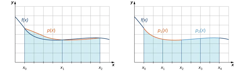
Simpson's Rule uses a quadratic through three consecutive sample points on each pair of subintervals; for sufficiently smooth functions it has a higher convergence order. It requires the number of subintervals $n$ to be even.

The approximation given by Simpson's Rule is:

$$\int_{a}^{b} f(x) dx \approx \frac{\Delta x}{3} \left[ f(x_0) + 4f(x_1) + 2f(x_2) + \ldots + 4f(x_{n-1}) + f(x_n) \right]$$

Open full-size image

On the left, one quadratic passes through three sampled points across two subintervals. On the right, the construction repeats with another quadratic. These pairs explain why composite Simpson integration needs an even number of subintervals. Compare the curved tops with the flat rectangles and straight trapezoid edges described above.

Gilbert Strang & Edwin Herman, OpenStax, Calculus Volume 2, Figure 3.16. · CC BY-NC-SA 4.0

Practical Use

These rules are particularly useful in Computer Science for solving problems that require numerical solutions, such as in simulations, optimization problems, and areas where the function cannot be integrated symbolically.

Implementation

Here are Python functions that implement each of these rules:

import numpy as np

def midpoint_rule(f, a, b, n):
    if isinstance(n, bool) or not isinstance(n, int) or n <= 0:
        raise ValueError("n must be a positive integer")
    dx = (b - a) / n
    x_mid = np.linspace(a + dx/2, b - dx/2, n)
    return np.sum(f(x_mid)) * dx

def trapezoid_rule(f, a, b, n):
    if isinstance(n, bool) or not isinstance(n, int) or n <= 0:
        raise ValueError("n must be a positive integer")
    dx = (b - a) / n
    x = np.linspace(a, b, n + 1)
    return dx/2 * np.sum(f(x[:-1]) + f(x[1:]))

def simpsons_rule(f, a, b, n):
    if isinstance(n, bool) or not isinstance(n, int) or n <= 0:
        raise ValueError("n must be a positive integer")
    if n % 2 == 1:
        raise ValueError("n must be even for Simpson's Rule")
    dx = (b - a) / n
    x = np.linspace(a, b, n + 1)
    y = f(x)
    return dx/3 * np.sum(y[0:-1:2] + 4*y[1::2] + y[2::2])

Notes:

• f is the integrand function.
• a and b are the limits of integration.
• n is the number of subintervals.
• dx is the width of each subinterval.
• For simpsons_rule, an even number of subintervals is necessary.

Error bounds and a reproducible check

For $a<b$, write $I=\int_a^b f(x)\,dx$. The composite-rule error bounds are

$$|I-M_n|\le\frac{K_2(b-a)^3}{24n^2},\qquad |I-T_n|\le\frac{K_2(b-a)^3}{12n^2},\qquad |I-S_n|\le\frac{K_4(b-a)^5}{180n^4}.$$

The first two require a continuous second derivative bounded in absolute value by $K_2$; Simpson requires a continuous fourth derivative bounded by $K_4$ and even $n$. Bounds describe discretization error, not floating-point rounding. Halving the step divides these bounds by 4 or 16. Simpson is exact for cubic polynomials in exact arithmetic, but is not universally more accurate for nonsmooth functions.

For $f(x)=x^2$ on $[0,1]$ and $n=2$, $M_2=5/16$, $T_2=3/8$, $S_2=1/3$, while $I=1/3$. The absolute errors are $1/48$, $1/24$, and zero, matching the bounds with $K_2=2$, $K_4=0$. To guarantee trapezoid error at most $10^{-4}$ here, choose $n\ge\lceil\sqrt{1/(6\cdot10^{-4})}\rceil=41$.

The implementation requires installed NumPy, finite bounds and a function that accepts an array and returns an array of the same shape. For a constant use lambda x: np.ones_like(x), not lambda x: 1. These are fixed-grid teaching routines, not adaptive singular-integral solvers.

f = lambda x: x**2
assert np.isclose(midpoint_rule(f, 0, 1, 2), 5/16)
assert np.isclose(trapezoid_rule(f, 0, 1, 2), 3/8)
assert np.isclose(simpsons_rule(f, 0, 1, 2), 1/3)

Compare results at $n,2n,4n$ to look for convergence, but agreement alone is not a certified bound: a grid can miss a narrow peak. Do not evaluate a singular endpoint with trapezoid or Simpson. Split or transform the integral first. For an infinite interval, truncation adds a separate tail error: replacing $\int_1^\infty x^{-2}\,dx$ by $\int_1^R x^{-2}\,dx$ loses exactly $1/R$, regardless of how fine the grid is.

My reading · Opened notes are remembered in this browser.