Log Loss in Machine Learning

Machine learning often involves optimization problems that aim to minimize or maximize a particular function, known as a loss function. Two of the most common loss functions are square loss and log loss. In this note, we'll delve into log loss by exploring a probability-based example and provide the mathematical foundations for understanding it better.

Mathematical Examination of Coin Flipping Scenario

Scenario Description

Consider the exercise of flipping a coin 10 times, aiming for a precise outcome of seven heads and three tails. Given three distinct coins with varying probabilities of landing heads ($p$) versus tails ($1-p$), we analyze which coin optimizes our chances of achieving the desired outcome.

Probability Analysis

For one particular ordered sequence containing seven heads and three tails, the probability is

$$p^7(1-p)^3.$$

If only the count matters and any ordering is allowed, the probability is

$$P(H=7)=\binom{10}{7}p^7(1-p)^3.$$

The binomial coefficient does not depend on $p$, so both expressions are maximized by the same value. Among coins with head probabilities 0.7, 0.5, and 0.3, the coin with $p=0.7$ gives the largest probability.

Optimization via Calculus

Objective Function Formulation

To generalize, we consider a coin with a variable head probability $p$. The goal becomes to find the value of $p$ that maximizes the likelihood function:

$$g(p) = p^7(1-p)^3$$

Optimization Technique

The maximization involves taking the derivative of $g(p)$ with respect to $p$, setting it to zero, and solving for $p$. This process yields:

$$\frac{dg}{dp} = 7p^6(1-p)^3 - 3p^7(1-p)^2 = 0$$

Solving the above equation reveals that $p=0.7$ is the optimal solution, aligning with our initial analysis.

Logarithmic Transformation and Simplification

Logarithmic Advantage

Transitioning to a logarithmic scale, $\log(g(p))$, simplifies the differentiation process due to the properties of logarithms, transforming products into sums and thereby easing computational efforts.

Derivation and Optimization

By optimizing the logarithm of $g(p)$, denoted $G(p)$, we find:

$$G(p) = \log(g(p)) = 7\log(p) + 3\log(1-p)$$

Differentiating and equating to zero yields:

$$\frac{dG}{dp} = \frac{7}{p} - \frac{3}{1-p} = 0$$

Solving for $p$ confirms the optimal probability as $p=0.7$.

Application of Log Loss in Machine Learning

In classification tasks within machine learning, log loss is defined inversely to $G(p)$:

$$\text{Log Loss} = -G(p)$$

This loss scores the predicted probabilities, not the fraction of correct class labels. Training minimizes it to fit those probabilities.

Why Use Logarithms in Log Loss?

Computational Simplicity

1. Derivatives of Sums vs Products: Calculating the derivative of a sum is computationally easier than that of a product. The product rule for derivatives gets increasingly complex with more terms. By taking the logarithm of the product, we can transform it into a sum, making it easier to differentiate.

   $$\text{Difficult: } \frac{d}{dx}(uv) = u'v + uv'$$ $$\text{Easier: } \frac{d}{dx}(\log (u) + \log (v)) = \frac{u'}{u} + \frac{v'}{v}$$

2. Avoiding Small Numbers: The product of probabilities can yield extremely small numbers that may not be computationally stable. Summing the logarithms of the individual probabilities avoids forming that tiny product in the first place.

Mathematical Formulae

• Complex Derivative without Logarithm: The derivative of the product becomes increasingly difficult to compute as more terms are added.

  $$\text{For example: } \frac{d}{dx}(uvw) = u'vw + uv'w + uvw'$$

• Simpler Derivative with Logarithm: Logarithmic differentiation simplifies this process.

  $$\text{For example: } \frac{d}{dx}(\log (u) + \log (v) + \log (w)) = \frac{u'}{u} + \frac{v'}{v} + \frac{w'}{w}$$

Concluding Insights

Log loss serves as a pivotal function in machine learning for assessing classification models. Its significance is amplified through the lens of probabilistic scenarios like coin flipping, where logarithmic transformations offer computational and mathematical conveniences. Numerical stability still depends on how those logarithms are evaluated, especially at probability endpoints.

From likelihood to a usable binary loss

Assume independent Bernoulli trials with a common $p$. Once seven heads and three tails have been observed, the same formula is a likelihood for the unknown $p$, not the probability that $p$ is true. On $0<p<1$, the natural logarithm is strictly increasing, so it preserves the maximizer. The negative log-likelihood $J=-G$ has

$$J'(p)=-\frac7p+\frac3{1-p},\qquad J''(p)=\frac7{p^2}+\frac3{(1-p)^2}>0.$$

It diverges at both boundaries, proving $p=0.7$ is the unique global minimum. Its value is about $6.108643$, or $0.610864$ per flip. With only heads, the optimum over $[0,1]$ would instead be the boundary $p=1$; an interior zero-derivative search would miss it.

For labels $y_i\in\{0,1\}$ and possibly different predicted probabilities $p_i$, binary cross-entropy is

$$\bar L=-\frac1n\sum_{i=1}^n\left[y_i\log p_i+(1-y_i)\log(1-p_i)\right].$$

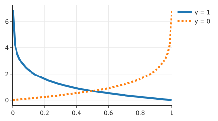
For $y=1$, predictions $0.9$ and $0.6$ both give the correct class at threshold $0.5$, but their losses are approximately $0.105361$ and $0.510826$. Log loss measures probability quality, not the fraction of correct hard labels. A confidently wrong probability $0.01$ incurs $4.605170$.

Open full-size image

The horizontal axis is the predicted probability p of class 1; the vertical axis is loss in natural-log units. Use the solid curve when y = 1 and the dotted curve when y = 0. Moving toward the confidently wrong endpoint makes the loss grow without bound, even though a hard classification records only one error.

Sam Lau, Joey Gonzalez & Deb Nolan, Learning Data Science, §19.4, © 2023. · CC BY-NC-ND 4.0

The endpoint convention $0\log0=0$ is a limit convention, not a valid floating-point multiplication. Giving the observed class zero probability incurs infinite loss. Compute sums of logs directly: taking a log after a probability product has underflowed cannot recover it. For probabilities strictly inside $(0,1)$, log1p(-p) evaluates $\log(1-p)$ accurately near zero. Clipping probabilities avoids infinities but changes the objective.

For binary labels and finite logits $z$, use the algebraically equivalent stable form

$$L(z,y)=\max(z,0)-yz+\log(1+e^{-|z|}).$$

In Python this is max(z, 0.0) - y*z + log1p(exp(-abs(z))). It returns about $1000$ for $(z,y)=(-1000,1)$ without overflowing. Thus logs help numerical stability only with a suitable implementation; neither arbitrary logarithms nor subtracting rounded sigmoid probabilities from one is automatically safe. The logistic-unit derivation explains why the logit gradient reduces to $\sigma(z)-y$.

My reading · Opened notes are remembered in this browser.