Limit Definitions

A limit describes the value a function approaches near an input. It depends on nearby behavior, so the value of the function at the input may be different or may not exist.

Finite Limit at a Finite Point

The statement

$$\lim_{x \to a} f(x)=L$$

means that $f(x)$ can be made arbitrarily close to $L$ by taking $x$ sufficiently close to $a$, while requiring $x\ne a$.

Formally, for every $\varepsilon>0$, there is a $\delta>0$ such that

$$0<|x-a|<\delta \quad\Longrightarrow\quad |f(x)-L|<\varepsilon.$$

The quantifier order matters: after a desired output tolerance $\varepsilon$ is chosen, one must find an input tolerance $\delta$ that works for every eligible $x$.

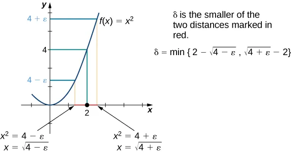
In 3Blue1Brown’s epsilon–delta lesson, follow the output tolerance band back to the input axis. Compare that geometric choice of δ with the algebraic bound in the next example.

Domain and a worked tolerance proof

For $f(x)=x^2$ near $2$, suppose the output must stay within $0.1$ of $4$: $|x^2-4|<0.1$. Keeping the input within $0.02$ of $2$, so $|x-2|<0.02$, is sufficient. Here $\varepsilon=0.1$ is the allowed output error, and $\delta=0.02$ is an input tolerance that guarantees it.

To see why this works, and prove $\lim_{x\to2}x^2=4$ for any output tolerance, factor the output error:

$$|x^2-4|=|x-2||x+2|.$$

First impose $|x-2|<1$, which gives $1<x<3$ and $|x+2|<5$. Given any $\varepsilon>0$, choose $\delta=\min(1,\varepsilon/5)$. Then $0<|x-2|<\delta$ implies $|x^2-4|<5\delta\le\varepsilon$. The preliminary bound removes the unknown $x$ from the tolerance choice.

Here $f:D\to\mathbb R$, and every condition on $x$ applies only to $x\in D$. The point $a$ must be an accumulation point of $D$: there are domain points other than $a$ arbitrarily close to it. Otherwise the implication would hold vacuously for every $L$. For a one-sided limit, domain points must approach from that side; at infinity, the domain must extend without bound in that direction.

Open full-size image

Start with the output band around 4, then trace its boundaries back to the x-axis. The smaller of the two input distances gives a safe symmetric δ. This geometric formula applies for 0 < ε < 4; the algebraic choice min(1, ε/5) above works for every ε > 0 and need not be the largest possible δ. Access for free at OpenStax.

Gilbert Strang & Edwin Herman, OpenStax, Calculus Volume 1, Figure 2.41. · CC BY-NC-SA 4.0

One-Sided Limits

The notation

$$\lim_{x\to a^-}f(x)=L \qquad\text{and}\qquad \lim_{x\to a^+}f(x)=L$$

restricts $x$ to values below or above $a$, respectively. This distinction is essential at jumps, endpoints, and piecewise boundaries. When domain points approach from both sides, the two-sided limit exists if and only if both one-sided limits exist and agree.

Limits at Infinity

The statement

$$\lim_{x\to\infty}f(x)=L$$

means that $f(x)$ approaches $L$ as $x$ becomes arbitrarily large. Formally, for every $\varepsilon>0$, there is a threshold $M$ such that

$$x>M \quad\Longrightarrow\quad |f(x)-L|<\varepsilon.$$

For $x\to-\infty$, the corresponding condition applies when $x<-M$.

Infinite Limits

The notation

$$\lim_{x\to a}f(x)=\infty$$

means that $f(x)$ eventually exceeds every positive bound as $x$ approaches $a$. It describes unbounded growth rather than a finite real-number limit. The notation $-\infty$ similarly describes values decreasing without bound.

For $\lim_{x\to a}f(x)=+\infty$, the precise requirement is: for every $B>0$, there exists $\delta>0$ such that $0<|x-a|<\delta$ implies $f(x)>B$. Merely being unbounded near $a$ is not enough: the inequality must hold for every sufficiently close domain point.

My reading · Opened notes are remembered in this browser.