Financial Markets and Mathematical Modeling

Suppose you pay a premium of 6 currency units for a European call option: the right, not the obligation, to buy one unit of an asset for 100 at expiry. This is a hypothetical contract for learning, not an investment recommendation or a currently offered product. Ignore transaction fees and discounting here, including interest on the premium paid upfront.

If the asset is worth 120 at expiry, the right to buy it for 100 has a payoff of 20. After subtracting the premium of 6, your profit is 14. If the asset is worth only 104, the payoff is still positive at 4, but the profit is −2. Receiving something at expiry does not necessarily mean making money.

Payoff and profit at expiry

Let $S_T$ be the asset price at expiry, $K=100$ the strike price, and $C_0=6$ the premium paid for this one-unit contract. Under the cost and time-value simplifications above:

$$\mathrm{payoff}_T=\max(S_T-K,0),\qquad \mathrm{profit}_T=\max(S_T-K,0)-C_0.$$

Asset price $S_T$	Payoff at expiry	Profit after premium
90	0	−6
104	4	−2
106	6	0
120	20	14

At 90, you let the option expire rather than exercise the right to pay 100. The break-even price is $K+C_0=106$. This table computes outcomes for given expiry prices; it does not tell us how likely those prices are or whether 6 is a fair premium today.

That second question needs a model of prices, uncertainty, time, and incentives. A financial model turns those assumptions into calculations so a trade or risk exposure is easier to reason about. It cannot remove market behavior that its assumptions leave out.

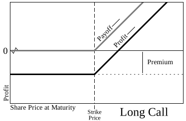Open full-size image

The grey payoff curve starts rising at the strike price; the black profit curve is lower by the premium, so it crosses zero later. In the example above, the bend is at 100, the vertical gap is 6, and break-even is 106. This schematic compares outcomes at expiry, not option prices before expiry. The Options Industry Council explanation gives the same strike-plus-premium break-even rule.

Gxti, Long call option (2009), Wikimedia Commons. · CC BY 3.0

From speculation to probability

In his 1900 thesis Théorie de la spéculation, Louis Bachelier modeled price changes with a stochastic process and derived an option-pricing formula. The work preceded modern mathematical finance and helped establish the idea that uncertain prices could be studied probabilistically rather than forecast one by one.

Earlier stories, such as Aristotle’s account of Thales reserving olive presses or Isaac Newton’s losses in the South Sea Bubble, are useful illustrations but not a continuous technical history of options or quantitative finance. They show that contingent claims and market overconfidence are old; they do not supply a modern pricing theory.

For the returns and risks of holding the underlying assets, start with the two-asset example in Returns, Diversification, and Portfolio Risk.

Options

The example buys a call and holds it to expiry. Other contract terms and positions change the rights and risks:

• a call concerns buying the underlying asset;
• a put concerns selling it;
• a European-style option is exercisable only at expiry;
• an American-style option is exercisable up to and including expiry.

Options can hedge risk or create leveraged exposure. For the purchased option above, the maximum loss is the premium of 6 under the stated simplifications. Written options and multi-leg positions can have very different loss profiles. “Options limit losses” is therefore true only for particular positions.

Black–Scholes–Merton

Black, Scholes, and Merton connected option values to a dynamically hedged portfolio under assumptions including frictionless trading, a specified price process (such as geometric Brownian motion), and continuous rebalancing. The 1997 Nobel Prize account describes this contribution to option pricing. The framework became a reference point for pricing and for thinking about no-arbitrage: related instruments should not offer a risk-free profit through inconsistent prices under the model’s trading assumptions.

No-Arbitrage and Binomial Option Pricing works through stock-and-bond replication and early-exercise decisions in a discrete model.

Real markets have jumps, changing volatility, transaction costs, discrete hedging, funding constraints, and liquidity risk. Traders therefore use extensions, implied-volatility surfaces, numerical methods, and judgment rather than treating one formula as a complete market description.

Quantitative trading

Edward Thorp and Jim Simons pioneered quantitative investment approaches. Public descriptions of private fund returns often mix gross and net performance, different date ranges, and unusually high fees. A famous annual percentage should not be compounded into a precise fortune without matching those definitions. Just as the call’s payoff differs from its profit, a fund’s return before fees differs from what an investor retains.

A testable rule, risk model, and execution process can be evaluated more clearly than a story about where price “should” go. None guarantees profit.

What models contribute

A model can:

• make assumptions explicit;
• connect prices across related instruments;
• estimate sensitivities and scenario losses;
• support repeatable decisions;
• reveal where observed prices disagree with the model.

The disagreement may be an opportunity, a bad assumption, stale data, or a risk the model omits. To investigate it, distinguish the contract’s payoff, the costs deducted from it, and the assumptions used to value it before expiry.

My reading · Opened notes are remembered in this browser.