Central Limit Theorem

The Central Limit Theorem is a fundamental statistical principle that describes the behavior of the average of a large number of identically distributed, independent random variables.

Definition

Let $X_1,X_2,\ldots$ be independent and identically distributed random variables with finite mean $\mu$ and finite, nonzero variance $\sigma^2$. The classical CLT states that the standardized sample mean converges in distribution to a standard normal random variable:

$$\frac{\sqrt{n}(\bar X_n-\mu)}{\sigma}\xrightarrow{d}N(0,1).$$

For large finite $n$, this is often used as the approximation

$$\bar{X}_n \approx N\left(\mu, \frac{\sigma^2}{n}\right).$$

where:

• $\bar{X}_n$ is the sample mean of the $n$ samples.
• $\mu$ is the population mean.
• $\sigma^2$ is the population variance.
• $n$ is the sample size.

Open full-size image

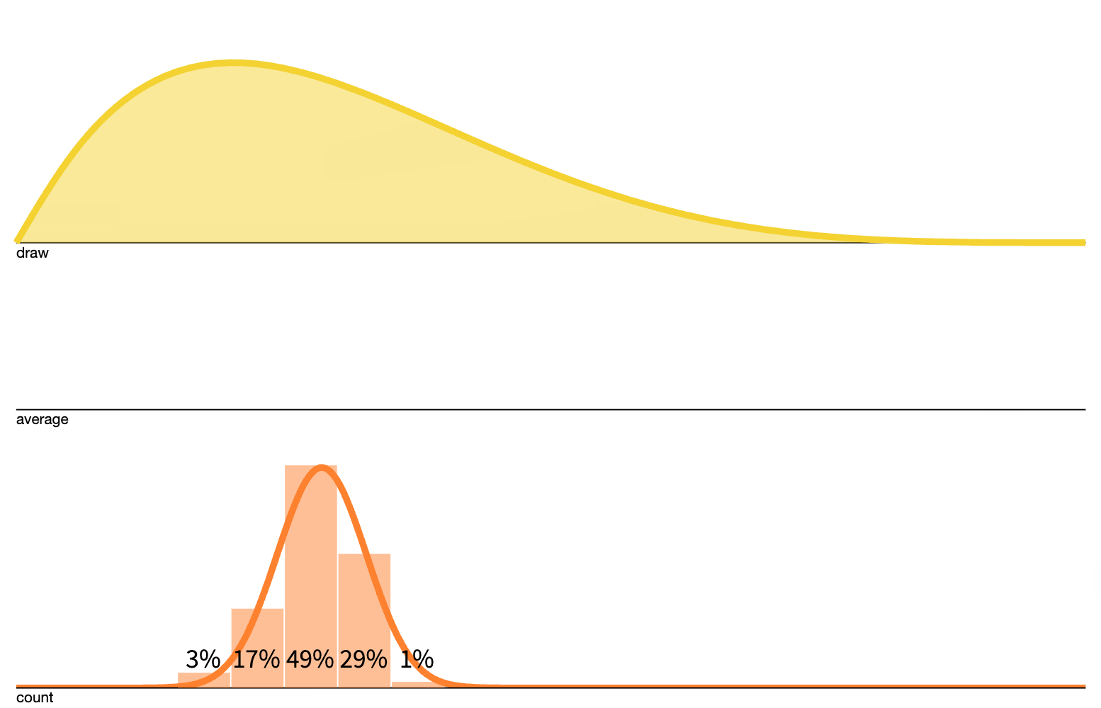
The source distribution is Beta(2, 5). The lower histogram collects repeated means of 15 independent draws; the orange line is a normal approximation. Compare its narrower, more symmetric shape with the skewed distribution above. The Python example below repeats the experiment with an exponential distribution.

Seeing Theory, Brown University, Central Limit Theorem; screenshot of the interactive plot, adapted from Philipp Plewa’s visualization. · Apache 2.0

Try the interactive experiment: keep α and β fixed, compare sample sizes 1 and 15, then increase Draws and press Sample again. Sample size changes the distribution of the mean; more repeated draws make its histogram more stable. The Theoretical option overlays the normal approximation when sample size exceeds 1.

Significance

• Normalization: Under the stated assumptions, the distribution of the sample mean is approximately normal for sufficiently large samples; how large depends on the population distribution.
• Predictability: It allows for making inferences about population means from sample means.
• Error Reduction: As the sample size increases, the standard error (SE) decreases, leading to more precise estimates.

Applications

• Polling and Surveys: Estimating population parameters such as voting intentions or consumer preferences from samples.
• Quality Control: Monitoring manufacturing processes where parameters like weight or volume are measured and controlled.
• Finance: Estimating the mean returns of different financial instruments to optimize investment portfolios.

Limitations

• Small Samples: The CLT may not hold well for small samples, especially if the population distribution is heavily skewed.
• Dependent Observations: The theorem assumes that the samples are independent. In cases where this assumption doesn't hold, the CLT may not apply.

Example Code in Python

To illustrate the CLT, consider the following Python code that simulates the distribution of the sample mean:

import numpy as np
import matplotlib.pyplot as plt

rng = np.random.default_rng(42)
sample_size = 30
num_samples = 5000

# Exponential data are strongly right-skewed, not normally distributed.
sample_means = [rng.exponential(scale=1, size=sample_size).mean()
                for _ in range(num_samples)]

# Plot distribution of sample means
plt.hist(sample_means, bins=30, color='blue', edgecolor='black', alpha=0.7)
plt.title('Distribution of Sample Means')
plt.xlabel('Sample Mean')
plt.ylabel('Frequency')
plt.show()

This example starts from a skewed exponential population. The histogram of repeated sample means becomes much more bell-shaped than the source distribution, which illustrates the approximation the CLT provides.

Why the scaling is square root of n

Independence makes the variance of a sum equal to the sum of variances. Dividing the sum by $n$ gives $\operatorname{Var}(\bar X_n)=n\sigma^2/n^2=\sigma^2/n$. Thus the mean fluctuates on the scale $\sigma/\sqrt n$. This variance identity is exact under the assumptions; the normal distribution is the asymptotic part of the theorem. The probability reference distinguishes standard deviation from standard error.

For the exponential population in the code, $\mu=\sigma=1$. At $n=30$, the mean has standard error $1/\sqrt{30}\approx0.183$. At $n=100$, it is 0.1, giving the normal approximation $P(0.804\le\bar X_{100}\le1.196)\approx0.95$. These are bounds for repeated sample means around a known population mean, not a confidence interval computed from one observed dataset. Quadrupling $n$ halves the standard error, rather than quartering it.

Cases where a large sample is not enough

There is no universal “$n=30$ is sufficient” rule. Rare events and strong skew can require much larger samples for useful tail probabilities. For a standard Cauchy population, the mean and variance do not exist, and the average of independent samples is still standard Cauchy: it does not concentrate or approach a normal distribution. See Siegrist’s derivation of the Cauchy sample-mean distribution. If all observations equal the same random variable $Y$, then $\bar X_n=Y$ for every $n$; dependence prevents the usual averaging gain.

The law of large numbers describes concentration around the mean; the CLT describes the shape after centering and rescaling. The observations themselves do not become normally distributed. When $\sigma$ is unknown, replacing it with a sample standard deviation adds estimation uncertainty: an exact Student t interval requires independent normal observations, while asymptotic studentized inference uses additional large-sample reasoning. Neither theorem repairs biased sampling or establishes that financial tail risk is normal.

Reference and Useful Links

• Central Limit Theorem (CLT): Definition and Key Characteristics

My reading · Opened notes are remembered in this browser.