Arrays and Dynamic Arrays

An array stores fixed-size slots contiguously, allowing the address of position $i$ to be computed from a base address and stride:

$$\operatorname{address}(i)=\operatorname{base}+i\cdot\operatorname{stride}.$$

This gives constant-time indexed access and strong spatial locality.

Open full-size image

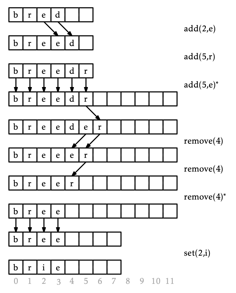
Compare each row with the one above it. An insertion in the middle shifts the suffix; adding at the end can use a spare slot. Asterisks mark resizing, where arrows show copies into a new backing array. Empty slots belong to capacity, not to the live sequence.

Pat Morin, Open Data Structures, Figure 2.1 (cropped from p. 34). · CC BY 2.5 CA

Static versus dynamic

• A static array has fixed capacity.
• A dynamic array tracks both length and capacity. When full, it allocates a larger backing array and copies existing slots.

Geometric capacity growth makes end append amortized $O(1)$ even though an individual resize costs $O(n)$. This is an aggregate guarantee, not a promise that every append has constant latency.

Operation costs

Operation	Typical cost
Read/write by index	$O(1)$
Sequential traversal	$O(n)$
Append at end	amortized $O(1)$
Pop from end	$O(1)$ without shrinking; otherwise amortized $O(1)$ with a suitable policy
Insert/delete near front or middle	$O(n)$ shifts
Search unsorted values	$O(n)$

Binary search is $O(\log n)$ only when ordering is maintained and random access is available; maintaining that order can make updates expensive.

Language boundary

Low-level typed arrays usually store homogeneous values inline. In CPython, a list uses contiguous reference slots; the referenced objects can be stored elsewhere and have different types. Other Python implementations may use different layouts.

Use boundary

Choose arrays for random access, compact iteration, sorting, matrices, and heap backing storage. Avoid front-of-array queue operations when frequent shifting would dominate.

Why the bounds hold

The table counts operations on fixed-size slots for a sequence of length $n$, as in Open Data Structures. Index arithmetic and moving or comparing one slot are treated as constant time; expensive element comparisons, object destruction, and allocation latency need separate accounting. Indexes in the address formula are zero-based and valid only from $0$ through $n-1$. Capacity is allocated storage; length is the number of live elements, with $0 \le n \le \text{capacity}$. Spare slots are not valid sequence elements.

For a doubling policy starting at capacity 1, appending eight items copies 1, 2, then 4 old slots at the three resizes: seven copies plus eight new writes. In general the geometric sum of copied capacities is less than $2m$ for $m$ appends from empty, so total work is $O(m)$. Growing by just one slot instead copies $1+2+\cdots+(m-1)$ slots, giving quadratic total work. The factor 2 is an explanatory policy, not Python's specified growth factor.

End removal requires no shifts. Its $O(1)$ bound assumes no backing-store resize: a shrinking implementation may copy $O(n)$ slots on one removal and offer only an amortized bound. Shrinking only when substantially underfull (for example, halving capacity at one-quarter occupancy) prevents alternating insertions and removals from repeatedly triggering large copies.

A concrete insertion

values = [10, 20, 30]
values.insert(1, 15)
assert values == [10, 15, 20, 30]
assert values.pop(1) == 15
assert values == [10, 20, 30]

Insertion shifts 20 and 30 right; deletion shifts them left. A saved index can therefore refer to a different element after mutation. At the low level, reallocation can also invalidate pointers into the old backing array; Python object references are distinct from such slot addresses. Python raises IndexError for an out-of-range indexed read and for pop() on an empty list.

Source

• Open Data Structures: Array-Based Lists

My reading · Opened notes are remembered in this browser.